A fast minimal residual solver for overlap fermions

Abstract

Computing quark propagators with overlap fermions requires the solution of a shifted unitary linear system. Jagels and Reichel have shown that for such systems it is possible to construct a minimal residual algorithm by short recurrences. The Jülich-Wuppertal group have found this algorithm to be the fastest among overlap solvers. In this paper we present a three-term recurrence for the Arnoldi unitary process. Using the new recurrence we construct a minimal residual solver which is the fastest among all Krylov subspace algorithms considered so far for the overlap inversion.

1 Introduction

Lattice theories with chiral quarks provide an accurate tool for studying the physics of strong interactions. The physical information of these theories is contained in quark propagators, which are then combined to construct meson, nucleon and even more complicated elementary particle propagators. Quark propagator computations amount to solving large linear systems of the type:

$$Dx=b$$ (1.1)

where $D\in\mathbb{C}^{N\times N}$ is a dense matrix operator representing the chiral Dirac operator on a regular four dimensional space-time lattice, $x,b\in\mathbb{C}^{N}$ are the quark propagator and its source.

More than a decade ago two formulations of chiral fermion theories were discovered: the domain wall fermions [1, 2] and overlap fermions [3]. These apparently different formulations are closely related to each other [4]. In particular, the truncated overlap variant of domain wall fermions [5] can be shown to be equivalent to overlap fermions in four dimensions at any lattice spacing [6]. Therefore, for computational purposes it is sufficient to consider the Neuberger Dirac operator, which is a shifted unitary matrix of the form [7]:

$$D=c_{1}\text{1\kern-2.41109ptl}+c_{2}V$$ (1.2)

where

$$V = D_{W}(D_{W}^{*}D_{W})^{-1/2}$$ (1.3)

$$c_{1} = (1+m)/2$$ (1.4)

$$c_{2} = (1-m)/2$$ (1.5)

Here $D_{W}$ is the Wilson-Dirac operator, which is a non-Hermitian sparse matrix. It is easy to see why $V$ is a unitary matrix: starting from the singular value decomposition of $D_{W}=X\Sigma Y^{*}$, one gets $V=XY^{*}$.

Another way to look into the Neuberger operator is to use operators $\Gamma_{5}=$diag$(I_{N/2},-I_{N/2})$ and $\hat{\Gamma}_{5}=$sign$(H_{W})$, where $H_{W}=\Gamma_{5}D_{W}$ is the Hermitian Wilson-Dirac operator. In this case it is easy to see that the overlap operator takes the form:

$$D=c_{1}\text{1\kern-2.41109ptl}+c_{2}\Gamma_{5}\hat{\Gamma}_{5}$$ (1.6)

This representation can be used to show that $D^{*}D$ commutes with $\Gamma_{5}$. As a result, $D^{*}D$ is block diagonal in the chiral basis of $\Gamma_{5}$. This observation has important applications: if we would like to solve linear systems with coefficient matrix $D^{*}D$ we can use Conjugate Gradients (CG) algorithm, which we know is optimal. Indeed, CG is very well suited for the molecular dynamics algorithm which generates the ensemble of gauge fields in lattice QCD with overlap fermions.

However, another important task is the computation of quark propagators which we consider here. This requires the solution of the linear systems of the type 1.1. One can still use CG on normal equations (CGNE) but this method may not be optimal in this case. In this paper we seek optimal solutions of the above system in the Krylov subspace:

$$x\in{\mathcal{K}}_{k}=span\{b,Db,\ldots,D^{k-1}b\}$$ (1.7)

It is well known that the generalized minimal residual method (GMRES) is the optimal method that can be constructed in this subspace. However, it is well known as well that the underlying Arnoldi process produces long recurrences, a feature which limits the benefits of the GMRES algorithm for large problems. Nonetheless, Jagels and Reichel [8] found that for shifted unitary systems it is possible to construct an Arnoldi process with short recurrences. The method, the shifted unitary minimal residual algorithm (SUMR) was shown by Jülich-Wuppertal group [9] to be the fastest linear solver for quark propagator computations.

Here we propose an approach, which is based on a three-term recurrence of the unitary Arnoldi process. This process is used to construct two optimal Krylov subspace methods: the shifted unitary orthogonal method (SUOM) and its geometric optimal counterpart SHUMR. We show that this algorithm converges faster then SUMR for all lattices and quark masses considered in this paper.

The paper is organised as follows: section 2 describes the new recurrence of the unitary Arnoldi process. Section 3 deals with the construction of the SUOM and SHUMR algorithms. In section 4 we compare directly these algorithms to SUMR and other Krylov subspace methods. Conclusions are drawn in section 5.

2 A three-term recurrence for the Arnoldi unitary process

Our aim in this section is to construct an orthogonal basis of the Krylov subspace 1.7 with as few operations as possible which will then be useful for the solution of the linear system 1.1. As a starting point we use the well-known Arnoldi process [10], which is essentially a modified Gram-Schmidt process, given in Algorithm 1.

Algorithm 1    Arnoldi process

  $q_{1}=b/||b||^{2}$

  for $~{}k=1,\ldots$ do

     $w=Vq_{k}$

     for $~{}j=1,\ldots,k$ do

        $h_{kj}=q_{j}^{*}w$

        $w:=w-q_{j}h_{jk}$

     end for

     $h_{k+1,k}=||w||_{2}$

     if $h_{k+1,k}=0$ then

        stop

     end if

     $q_{k+1}=w/h_{k+1,k}$

  end for

After $k$ steps of this algorithm, the next unnormalized Arnoldi vector is given by:

$${\tilde{q}}_{k+1}=Vq_{k}-\sum_{j=1}^{k}q_{j}h_{jk}$$ (2.1)

The right hand side contains a linear combination over all computed Arnoldi vectors. This makes the overall complexity of the algorithm to grow quadratically with $k$. Moreover, the computer memory grows linearly with $k$, a requirement which is often prohibitive and thus undesirable for large problems like ours.

Fortunately, for unitary matrices one can do better. After $k$ steps of Algorithm 1 we can write:

$$VQ_{k}=Q_{k}H_{k}+h_{k+1,k}q_{k+1}e_{k}^{T}\equiv Q_{k+1}{\tilde{H}}_{k}$$ (2.2)

where $Q_{k}=[q_{1},\ldots,q_{k}]$ is the matrix of orthonormal Arnoldi vectors, $H_{k}$ is an $k\times k$ upper Hessenberg matrix and ${\tilde{H}}_{k}$ is a $k+1\times k$ matrix obtained by appending the row $h_{k+1,k}e_{k}^{T}$ to the matrix $H_{k}$.

Proposition 2.1

${\tilde{H}}_{k}$ has orthonormal columns.

Proof. Multiplying both sides of 2.2 from left by $Q_{k}^{*}$ we get:

$$Q_{k}^{*}VQ_{k}=H_{k}$$ (2.3)

Multiplying both sides of 2.2 from left again but now by $(VQ_{k})^{*}$ we get:

$$I_{k}=Q_{k}^{*}V^{*}Q_{k}H_{k}+h_{k+1,k}(q_{k+1}^{*}VQ_{k})^{*}e_{k}^{T}$$ (2.4)

From 2.3 and 2.2 one gets $Q_{k}^{*}V^{*}Q_{k}=H_{k}^{*}$ and $q_{k+1}^{*}VQ_{k}=h_{k+1}e_{k}^{T}$. Thus, we find that:

$$I_{k}=H_{k}^{*}H_{k}+h_{k+1,k}^{2}e_{k}e_{k}^{T}={\tilde{H}}_{k}^{*}{\tilde{H}}_{k}$$ (2.5)

which proves the proposition. $\Box$

Corollary 2.2

From 2.5 it is clear that $H_{k}$ is a unitary matrix if its last column is normalised.

This property was used be Jagels and Reichel to write $H_{k}$ as a product of $k$ elementary Givens rotations, which are then exploited to construct a coupled two-term recurrence Arnoldi algorithm (see Algorithm 3.1 of [8]). They note that solving the coupled recurrences would still lead to an algorithm where all vectors are required.

In contrast to their work, we give an algorithm which is defined by short recurrences. We start by noting that the LU-decomposition of the upper Hessenberg matrix $H_{k}$ can be written in the form:

$$H_{k}=L_{k}U_{k}^{-1}$$ (2.6)

where $L_{k}$ is a lower bidiagonal matrix and $U_{k}$ is upper triangular. For our convenience, we take the diagonal elements of $U_{k}$ to be one. Substituting this decomposition into 2.5, multiplying the result from the right by $U_{k}$ and from the left by $U_{k}^{*}$ we get:

$$U_{k}^{*}U_{k}=L_{k}^{*}L_{k}+h_{k+1,k}^{2}e_{k}e_{k}^{T}$$ (2.7)

Since the right hand side is a tridiagonal Hermitian matrix so must be the left hand side. Hence, $U_{k}$ should be upper bidiagonal. This decomposition, eq. 2.6 was used for the first time by Rutishauser to compute the eigenvalues of orthogonal Hessenberg matrices [11]. We can easily extend this decomposition for the matrix $\tilde{H}_{k}$:

$$\tilde{H}_{k}=\hat{L}_{k}U_{k}^{-1},~{}~{}~{}~{}\hat{L}_{k}=L_{k}+l_{k+1,k}e_{k}^{T}$$ (2.8)

which gives $h_{k+1,k}=l_{k+1,k}$.

Multiplying both sides of 2.2 by $U_{k}$ we get:

$$VQ_{k}U_{k}=Q_{k}L_{k}+l_{k+1,k}q_{k+1}e_{k}^{T}.$$ (2.9)

This way, the next Arnoldi vector can be computed using:

$$l_{k+1,k}~{}q_{k+1}=(V-l_{kk}I)q_{k}+Vq_{k-1}u_{k-1,k}$$ (2.10)

where

$$u_{k-1,k}=-\frac{q_{k-1}^{*}Vq_{k}}{q_{k-1}^{*}Vq_{k-1}}$$ (2.11)

and

$$l_{kk}=q_{k}^{*}Vq_{k}+q_{k}^{*}Vq_{k-1}u_{k-1,k}$$ (2.12)

These expressions allow us to construct the three-term recurrence Arnoldi unitary process as given in Algorithm 2.

Algorithm 2    Arnoldi unitary process

  $u_{01}=0$, $q_{1}=b/||b||^{2}$

  for $~{}k=1,\ldots n$ do

     $w_{k}=Vq_{k}$

     $u_{k-1,k}=-(q_{k-1}^{*}w_{k})/(q_{k-1}^{*}w_{k-1})$          (for $k>1$)

     $l_{kk}=q_{k}^{*}w_{k}+q_{k}^{*}w_{k-1}u_{k-1,k}$

     $w_{k+1}=w_{k}-l_{kk}q_{k}+u_{k-1,k}w_{k-1}$

     $l_{k+1,k}=||w_{k+1}||_{2}$

     if $l_{k+1,k}=0$ then

        stop

     end if

     $q_{k+1}=w_{k+1}/l_{k+1,k}$

  end for

Note that the algorithm needs an additional inner product than the usual (eg. Lanczos) three-term recurrence algorithms. The reason is the appearance of the matrix $V$ both in the diagonal and subdiagonal terms of 2.10. The algorithm is equivalent to the normal Arnoldi algorithm in exact arithmetic as the following proposition shows:

Proposition 2.3

Given $q_{1}$ and $V$ unitary the unitary Arnoldi process, Algorithm 2 generates the orthonormal vectors $Q_{k}$, the lower and upper bidiagonal matrices $L_{k}$, $U_{k}$ such that $\hat{L}_{k+1}U_{k}^{-1}$ is a matrix with orthonormal columns.

Proof. The algorithm produces orthonormal vectors $Q_{k}$ and matrices $L_{k}$ and $U_{k}$ such that equations 2.9 is satisfied. Multiplying both sides of these equations by $U_{k}^{-1}$ we get new equations where $L_{k}U_{k}^{-1}$ is upper Hessenberg. From Proposition 2.1 follows that $\tilde{H}_{k}$ and thus $\hat{L}_{k+1}U_{k}^{-1}$ is a matrix with orthonormal columns. $\Box$

Remark 2.4

Both Arnoldi processes produce the same basis for the Krylov subspace but Algorithm 2 is more efficient: its complexity is linear in $k$ and its computer memory requirement is constant at each step $k$.

3 Optimal Krylov subspace methods for the overlap inversion

The overlap operator is a non-Hermitian matrix operator. For such matrices GMRES is knwon to be the optimal algorithm. We call this class of algorithms geometrically optimal. Another algorithm which can be used for such problems is the full orthogonalisation method (FOM). In this case the $k^{\text{th}}$ residual vector,

$$r_{k}=b-Dx_{k}$$ (3.1)

lies orthogonal to the Krylov subspace ${\cal K}_{k}$. Because of this algebraic property we call this class of algorithms algebraically optimal. It can be shown that when the norm-minimising process of GMRES is converging rapidly, the residual norms in the corresponding Galerkin process of FOM exhibit similar behaviour [12].

Both methods GMRES and FOM use the Arnoldi process to generate the iterates. In this section we will use the Arnoldi unitary process to construct two algorithms: the first one is the specialisation of FOM to shifted unitary systems, whereas the second is the specialisation of GMRES to these systems.

3.1 A full orthogonalisation strategy

We seek the solution in the Krylov subspace spanned by the Arnoldi vectors, i.e.

$$x_{k}=Q_{k}y_{k},~{}~{}~{}~{}y_{k}\in\mathbb{C}^{k}$$ (3.2)

Assuming for simplicity that $\left\|b\right\|=1$, and using eq. 3.1 the residual vector will be,

$$r_{k}=Q_{k}e_{1}-DQ_{k}y_{k}$$ (3.3)

Using the definition of D, eq. 1.2 and the relation 2.9 we get:

$$r_{k}=Q_{k}e_{1}-Q_{k+1}(c_{1}\tilde{\text{1\kern-2.41109ptl}}_{k}+c_{2}\hat{L}_{k}U_{k}^{-1})y_{k}$$ (3.4)

where $\tilde{\text{1\kern-2.41109ptl}}_{k}$ is obtained by appending a row of $k$ zeros to the unit matrix 1l. Projecting this equation onto the Krylov subspace ${\cal K}_{k}$ one has:

$$o=e_{1}-(c_{1}\text{1\kern-2.41109ptl}_{k}+c_{2}L_{k}U_{k}^{-1})y_{k}$$ (3.5)

or equivalently:

$$(c_{1}U_{k}+c_{2}L_{k})z_{k}=e_{1},~{}~{}~{}z_{k}=U_{k}^{-1}y_{k}$$ (3.6)

Note that the matrix on the left hand side is tridiagonal and we can write:

$$T_{k}z_{k}=e_{1},~{}~{}~{}T_{k}=c_{1}U_{k}+c_{2}L_{k}$$ (3.7)

The LU decomposition of the matrix $T_{k}$ is denoted by $T_{k}={\tilde{L}}_{k}{\tilde{U}}_{k}$. Hence the solution can be written as:

$$z_{k}={\tilde{U}}_{k}^{-1}{\tilde{L}}_{k}^{-1}e_{1}={\tilde{U}}_{k}^{-1}\begin{pmatrix}{\tilde{L}}_{k-1}^{-1}e_{1}\\ \alpha_{k}\end{pmatrix}=\begin{pmatrix}z_{k-1}\\ 0\end{pmatrix}+\alpha_{k}{\tilde{U}}_{k}^{-1}e_{k}$$ (3.8)

where

$$\alpha_{k}=e_{k}^{T}T_{k}^{-1}e_{1}=e_{k}^{T}{\tilde{L}}_{k}^{-1}e_{1}$$ (3.9)

Then from $x_{k}=Q_{k}U_{k}z_{k}$ with $Q_{k}U_{k}=[Q_{k-1}U_{k-1},q_{k}+q_{k-1}u_{k-1,k}]$ and from the recurrence for $z_{k}$, eq. 3.8 we get:

$$x_{k}=Q_{k-1}U_{k-1}z_{k-1}+\alpha_{k}~{}Q_{k}U_{k}{\tilde{U}}_{k}^{-1}e_{k}$$ (3.10)

Finally, denoting,

$$w_{k}=Q_{k}U_{k}{\tilde{U}}_{k}^{-1}e_{k}$$ (3.11)

we have:

$$x_{k}=x_{k-1}+\alpha_{k}w_{k}$$ (3.12)

Using this result and the definition of the residual vector, eq. 3.1 we get:

$$r_{k}=r_{k-1}-\alpha_{k}Dw_{k}$$ (3.13)

Using matrices $\tilde{L}_{k},\tilde{U}_{k}$ it is easy to show (see Appendix A) that the following recurrences hold:

$$w_{k} = q_{k}+q_{k-1}u_{k-1,k}+\frac{\gamma_{k-1}}{{\tilde{l}}_{k-1,k-1}}w_{k-1}$$ (3.14)

$$\alpha_{k} = \frac{\beta_{k-1}}{{\tilde{l}}_{kk}}\alpha_{k-1}$$ (3.15)

$${\tilde{l}}_{kk} = c_{1}+c_{2}l_{kk}-\frac{\beta_{k-1}\gamma_{k-1}}{{\tilde{l}}_{k-1,k-1}}$$ (3.16)

where $\beta_{k}=-c_{2}l_{k+1,k}$ and $\gamma_{k}=-c_{1}u_{k,k+1}$.

In this way we have specified the iterations for this linear solver, which is called the shifted unitary orthogonal method or SUOM. Below we give the MATLAB function SUOM.m. The input is the right hand side vector $b$, the exact solution $x_{0}$, the unitary matrix $V$, the real constants $c_{1}$ and $c_{2}$, the tolerance $tol$ and the maximum number of iterations $imax$. The output is the error norm history $rr$ and the solution $x$.

⬇

function [rr,x] = SUOM(b,x0,V,c1,c2,tol,imax);

b=b(:);

N=max(size(b));

vzero=zeros(N,1);

x=vzero;

r=b;

rho = norm(r);

rnorm=rho;

rr=norm(x0);

alpha = rho;

u12=0;

beta=1;

L11_tilde=1;

q=r/rho;

q_old=vzero; v_old=vzero; w_old=vzero; s_old=vzero;

counter = 1;

while ( (rnorm > tol) & (counter<=imax) );

v=V*q;

if (counter > 1),

u12=-(q_old’*v)/(q_old’*v_old);

␣␣end

␣␣gamma=-c1*u12;

␣␣L11=(q’*v)+u12*(q’*v_old);

␣␣q_tilde=v-L11*q+u12*v_old;

␣␣L21=norm(q_tilde);

␣␣if␣(L21<=tol),␣break,␣end;

␣␣w=q+q_old*u12+w_old*gamma/L11_tilde;

␣␣s=c1*(q+q_old*u12)+c2*(v+v_old*u12)+s_old*gamma/L11_tilde;

␣␣L11_tilde=c1+c2*L11-beta*gamma/L11_tilde;

␣␣alpha=alpha*beta/L11_tilde;

␣␣x=x+w*alpha;

␣␣r=r-s*alpha;

␣␣q_old=q;␣v_old=v;␣w_old=w;␣s_old=s;

␣␣q=q_tilde/L21;

␣␣beta=-c2*L21;

␣␣rnorm=norm(r);

␣␣rr=[rr;norm(x0-x)];

␣␣counter++;

end

Note that the code can be trivially changed in order to get the residual error norm instead of the error norm, or to use $x_{0}$ as a starting guess by defining the starting residual error as $r=b-Dx_{0}$.

Another advantage of our MATLAB code is its easy inclusion into a C++ code which uses uBLAS libraries for inner products and Euclidean norms . We have used these libraries to construct such a C++ function for use with overlap fermions. In this case, the matrix-vector multiplication is an external routine which applies the inverse square root of $D_{W}^{*}D_{W}$ to the current Arnoldi vector $q$ followed by a $D_{W}$ multiplication.

3.2 A minimal residual strategy

As in the previous case our starting point is the Krylov subspace ${\cal K}_{k}$. But instead of projecting the residual vector we seek the minimum of its 2-norm on this subspace. The solution in this case is denoted by $\tilde{x}_{k}$ and is written formally as a solution of a Least Squares Problem (LSP):

$$\tilde{x}_{k}=\text{arg}\min_{x\in{\cal K}_{k}}\left\|b-Dx\right\|_{2}$$ (3.17)

Requiring $x=Q_{k}y$ and using eq. 3.4 we get:

$$\tilde{y}_{k}=\text{arg}\min_{y\in\mathbb{C}^{k}}\left\|Q_{k+1}~{}[e_{1}-(c_{1}\tilde{\text{1\kern-2.41109ptl}}_{k}+c_{2}\hat{L}_{k}U_{k}^{-1})y]~{}\right\|_{2}$$ (3.18)

Since Arnoldi vectors are orthonormal, the matrix $Q_{k+1}$ can be ignored and we end up with a much smaller LSP. Note that the matrix ${\tilde{H}}_{k}=\hat{L}_{k}U_{k}^{-1}$ has orthonormal columns (see Proposition 2.1), a property which can be used to get a short recurrence algorithm as in the case of the SUMR algorithm [8]. However, as in the case of SUOM, we follow a strategy that involves a tridiagonal matrix in the LSP. This way the solution of the smaller problem is given by:

$$\tilde{z}_{k}=\text{arg}\min_{z\in\mathbb{C}^{k}}\left\|e_{1}-(c_{1}U_{k}+c_{2}\hat{L}_{k})z\right\|_{2},~{}~{}~{}~{}\tilde{y}_{k}=U_{k}\tilde{z}_{k}$$ (3.19)

where

$$c_{1}U_{k}+c_{2}\hat{L}_{k}=\begin{pmatrix}T_{k}\\ \nu e_{k}^{T}\\ \end{pmatrix}\equiv\tilde{T}_{k},~{}~{}~{}\nu=c_{2}~{}l_{k+1,k}$$ (3.20)

In order to compute the iterates from those of the SUOM algorithm we split the solution vector as follows:

$$\tilde{z}_{k}=z_{k}+\xi_{k}$$ (3.21)

Using equations 3.7-3.9 we get:

$$\xi_{k}=\text{arg}\min_{\xi\in\mathbb{C}^{k}}\left\|\nu\alpha_{k}e_{k+1}+\tilde{T}_{k}\xi\right\|_{2}$$ (3.22)

We solve this LSP by QR factorization of the matrix $\tilde{T}_{k}$:

$$\tilde{T}_{k}=O_{k}^{*}\tilde{R}_{k},~{}~{}~{}\tilde{R}_{k}=\begin{pmatrix}R_{k}\\ 0\\ \end{pmatrix}$$ (3.23)

with $O_{k}$ being a $k+1\times k+1$ unitary matrix and $R_{k}$ an upper tridiagonal matrix. Therefore we have:

$$\xi_{k}=\text{arg}\min_{\xi\in\mathbb{C}^{k}}\left\|\nu\alpha_{k}O_{k}e_{k+1}+\tilde{R}_{k}\xi\right\|_{2}$$ (3.24)

As it is usual in this case, the unitary matrix can be constructed using Givens rotations. At step $k$ one can express it in the form:

$$O_{k}=G_{k}\begin{pmatrix}O_{k-1}&0\\ 0&1\\ \end{pmatrix},~{}~{}~{}~{}G_{k}=\begin{pmatrix}I_{k-1}&&\\ &c_{k}&s_{k}\\ &-\bar{s}_{k}&c_{k}\\ \end{pmatrix},~{}~{}~{}c_{k}^{2}+\left|s_{k}\right|^{2}=1$$ (3.25)

From this it is clear that:

$$O_{k}e_{k+1}=s_{k}e_{k}+c_{k}e_{k+1}$$ (3.26)

which gives:

$$\min_{\xi\in\mathbb{C}^{k}}\left\|\nu\alpha_{k}O_{k}e_{k+1}+\tilde{R}_{k}\xi\right\|_{2}=\min_{\xi\in\mathbb{C}^{k}}\left\|\nu\alpha_{k}s_{k}e_{k}+R_{k}\xi\right\|_{2}+\left|\nu\alpha_{k}c_{k}\right|$$ (3.27)

The right hand side is minimal if its first term is minimal. If we assume that $R_{k}$ has full rank then this term must vanish. In this case the solution is given by:

$$\xi_{k}=-R_{k}^{-1}e_{k}\nu\alpha_{k}s_{k}$$ (3.28)

Using 3.18-3.21, the solution to the original problem can be written as:

$$\tilde{x}_{k}=Q_{k}U_{k}z_{k}+Q_{k}U_{k}\xi_{k}=x_{k}+Q_{k}U_{k}\xi_{k}\equiv x_{k}+\hat{x}_{k}$$ (3.29)

where

$$\hat{x}_{k}=-Q_{k}U_{k}R_{k}^{-1}e_{k}\nu\alpha_{k}s_{k}$$ (3.30)

In order to simplify the expression we define the matrix $P_{k}$:

$$P_{k}=[p_{1},\ldots,p_{k}]=Q_{k}U_{k}R_{k}^{-1}$$ (3.31)

and denote $\omega_{k}=\nu\alpha_{k}s_{k}$. This way we have:

$$\hat{x}_{k}=-\omega_{k}p_{k}$$ (3.32)

To complete the algorithm one should write the recurrence on $p_{k}$. Multiplying both sides of 3.31 by $R_{k}$ from the right we get $P_{k}R_{k}=Q_{k}U_{k}$, which gives:

$$p_{k}\mu_{k}+p_{k-1}\varepsilon_{k}+p_{k-2}\theta_{k}=q_{k}+q_{k-1}u_{k-1,k}$$ (3.33)

where by $\mu_{k},\varepsilon_{k}$ and $\theta_{k}$ we denote the only non-zero entries of the last column of $R_{k}$. From this equation we get:

$$p_{k}=(q_{k}+q_{k-1}u_{k-1,k}-p_{k-1}\varepsilon_{k}-p_{k-2}\theta_{k})/\mu_{k}$$ (3.34)

This completes the description of the method, which we call SHUMR in order to distinguish it from the SUMR algorithm. The details of the QR decomposition are given in Appendix B. The MATLAB code of the algorithm is listed below. It differs from the SUOM code with lines between “$start~{}~{}added~{}~{}lines$” and “$end~{}~{}added~{}~{}lines$”. One can make here the same remarks as made in the case of the SUOM.m function. In particular, the code can be easily modified into a C++ code using uBLAS libraries.

⬇

function [rr,x] = SHUMR(b,x0,V,c1,c2,tol,imax);

b=b(:);

N=max(size(b));

vzero=zeros(N,1);

x=vzero;

r=b;

rho = norm(r);

rnorm=rho;

rr=norm(x0);

alpha = rho;

u12=0;

beta=1;

L11_tilde=1;

q=r/rho;

q_old=vzero; v_old=vzero; w_old=vzero; s_old=vzero;

% start added lines

c_km1=1; s_km1=0; c_km2=0; s_km2=0;

p1=vzero; p2=vzero; Dp1=vzero; Dp2=vzero;

% end added lines

counter = 1;

while ( (rnorm > tol) & (counter<=imax) );

v=V*q;

if (counter > 1),

u12=-(q_old’*v)/(q_old’*v_old);

␣␣end

␣␣gamma=-c1*u12;

␣␣L11=(q’*v)+u12*(q’*v_old);

␣␣q_tilde=v-L11*q+u12*v_old;

␣␣L21=norm(q_tilde);

␣␣if␣(L21<=tol),␣break,␣end;

␣␣w=q+q_old*u12+w_old*gamma/L11_tilde;

␣␣s=c1*(q+q_old*u12)+c2*(v+v_old*u12)+s_old*gamma/L11_tilde;

␣␣L11_tilde=c1+c2*L11-beta*gamma/L11_tilde;

␣␣alpha=alpha*beta/L11_tilde;

␣␣x=x+w*alpha;

␣␣r=r-s*alpha;

␣␣q_old=q;␣v_old=v;␣w_old=w;␣s_old=s;

␣␣q=q_tilde/L21;

␣␣beta=-c2*L21;

␣␣rnorm=norm(r);

%␣start␣added␣lines

␣␣t11=c1+c2*L11;

␣␣mu=t11*c_km1+gamma*conj(s_km1)*c_km2;

␣␣nu=c2*L21;

␣␣if␣(mu␣!=␣0),

␣␣␣␣c_k=abs(mu)/sqrt(abs(mu)*abs(mu)+abs(nu)*abs(nu));

␣␣␣␣s_k=conj(c_k*nu/mu);

␣␣else

␣␣␣␣c_k=0;

␣␣␣␣s_k=1;

␣␣end

␣␣omega=nu*alpha*s_k;

␣␣mu_k=c_k*mu+s_k*nu;

␣␣eps=t11*s_km1-gamma*c_km1*c_km2;

␣␣theta=-gamma*s_km2;

␣␣p=(q+q_old*u12-p1*eps-p2*theta)/mu_k;

␣␣Dp=(c1*(q+q_old*u12)+c2*(v+v_old*u12)-Dp1*eps-Dp2*theta)/mu_k;

␣␣rnorm_p=norm(r+omega*Dp);

␣␣xp=x-omega*p;

␣␣c_km2=c_km1;␣s_km2=s_km1;␣p2=p1;␣Dp2=Dp1;

␣␣c_km1=c_k;␣s_km1=s_k;␣p1=p;␣Dp1=Dp;

%␣end␣added␣lines

␣␣rr=[rr;norm(x0-xp)];

␣␣counter++;

end

3.3 A numerical example

We note that SUMR and SHUMR algorithms differ in the underlying Arnoldi process: the SUMR algorithm uses two coupled two-term recurrences which, when are solved, yield the usual long recurrence of the Arnoldi algorithm; the SHUMR algorithm uses a three-term recurrence. In principle, it is possible to compare theoretically the effect of such a difference, but this goes beyond the purpose of this paper. We have chosen instead a direct numerical comparison in case of overlap fermions, since this is of great importance for practical lattice computations. Before we do so we give a first example in the case of a small, i.e. $200\times 200$ unitary matrix.

The example is similar to Example 2 of the paper of Jagels and Reichel [8]. Let $W$ unitary matrix of the order $200$ resulting from the QR decomposition of a matrix with random elements in the interval $(0,1)$. Let $\Lambda$ be a diagonal unitary matrix with elements $\lambda_{k}=e^{i\theta_{k}}$ where

$$\theta_{k}=\pi(k-1)/6,~{}~{}~{}~{}1\leq k\leq 6$$

and the rest is randomly distributed in the interval $(-\pi/4,\pi/4)$. Then, the unitary matrix $V$ is defined by:

$$V=W\Lambda W^{*}$$

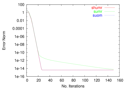
We have tested SHUMR,SUOM,SUMR algorithms for solving the linear system $Ax=b$ where $A=c_{1}\text{1\kern-2.41109ptl}+c_{2}V$ with $c_{1}=1.05$ and $c_{2}=1$ and random right hand side $b$. The results are shown in Figure 1. We observe that SHUMR and SUOM lie on top of each other (in this scale) and converge linearly until they stagnate below $10^{-14}$. On the other hand the convergence rate of the SUMR algorithm slows down when the value of the error norm is around $10^{-10}$. It is not clear why SUMR differs in this way from SHUMR and SUOM in this particular example.

Figure 1: Comparison of SHUMR,SUOM,SUMR algorithms for solving a small shifted unitary linear system as described in the text.

4 Comparison of algorithms for the overlap inversion

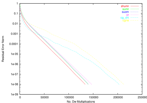
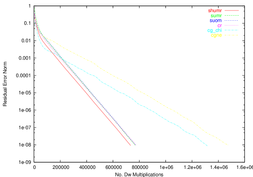
In this section we compare the convergence of SUMR, SUOM and SHUMR algorithms in the case of overlap fermions. SUMR and SHUMR are geometrically optimal algorithms for shifted linear systems, whereas SUOM is algebraically optimal in the sense defined above. For completeness we display the convergence of Conjugate Residuals (CR), Conjugate Gradients on Normal Equations (CGNE) and a special variation of CGNE which we call CG-CHI. The latter exploits the fact that $D^{*}D$ is block diagonal and solves simultaneously the two decoupled chiral systems.

Note that the computation of $D$ as applied to a vector is a numerical problem, which is by now well researched. A good review of these methods can be found in [13]. We use the Lanczos method [14, 15], in the double pass version and without $H_{W}$-eigenvalue projection.

In the figures below we show the convergence of algorithms as a function of Wilson matrix-vector multiplication number on $8^{3}16$ quenched lattices at various couplings and quark masses.

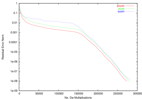
Figure 2 compares all above mentioned algorithms for quark mass $m=0.05$ at $\beta=6$ and $\beta=5.7$. The first observation is that SHUMR, SUMR, SUOM and CR are more efficient than CGNE and CG-CHI algorithms. This is observed by the other groups as well [9]. Hence, we decided not run these algorithms further for smaller quark masses. The second observation is that SUMR, SUOM and CR converge neck-to-neck with CR being slightly worse at $\beta=6$. The third observation is that SHUMR converges $10-15\%$ faster than SUMR and SUOM.

Figure 2: Convergence history of various solvers on background gauge fields at $\beta=6$ (upper part) and $\beta=5.7$ (lower part) and quark mass $m=0.05$

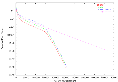
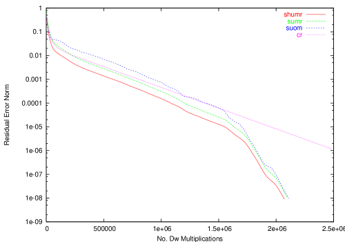
Figure 3: Convergence history of SUMR, SUOM, SHUMR and CR on background gauge fields at $\beta=6$ (upper part) and $\beta=5.7$ (lower part) and quark mass $m=0.01$

Figure 3 compares the algorithms remaining in race for the quark mass $m=0.01$ at $\beta=6$ and $\beta=5.7$. At this lighter mass we observe a superlinear convergence rate of SHUMR, SUMR and SUOM: the rate increases around residual norm $10^{-3}$ at $\beta=6$ and around $10^{-5}$ at $\beta=5.7$. This is to be contrasted to the linear convergence of CR. A second observation at this mass is the emergence of the pattern that SHUMR converges faster than SUMR and the latter converges faster than SUOM. This pattern is confirmed in Figure 4 where the quark mass is lowered to $m=0.005$.

Figure 4: Convergence history of SUMR, SUOM and SHUMR on background gauge fields at $\beta=6$ and quark mass $m=0.005$

Hence, the best algorithms are the optimal algorithms SHUMR and SUMR with SHUMR converging $10-15\%$ faster in all cases. Although both algorithms minimise the residual vector norm they differ in the underlying Arnoldi process. The nature of short recurrences employed by SHUMR may impact numerical properties of the algorithm. Hence, generated Krylov subspaces are different and we may conclude that SHUMR explores it more efficiently. However, at present we have no theoretical tool to characterise the difference.

5 Conclusions

In this paper we have presented two iterative solvers which are based on a new Arnoldi type algorithm for shifted unitary systems. The SUOM solver constructs residual vectors which are orthogonal to the Krylov subspace. The SHUMR solver minimises the residual vector over the generated Krylov subspace. Both algorithms are short recurrence specialisations of FOM and GMRES for shifted unitary systems. Taking into account the SUMR algorithm of Jagels and Reichel [8], the short recurrence algorithms for such systems are hardly a new result. But, it is somewhat surprising that the SHUMR algorithm performs better than SUMR on the examples shown in this paper. In particular, we presented a new Arnoldi unitary process, Algorithm 2, which is intrinsically a short recurrence process, a result which appears for the first time.

On the application level we conclude that SHUMR algorithm outperforms all other knwon iterative solvers for quark propagator computations with overlap fermions. The MATLAB codes of SUOM and SHUMR algorithms given here allow an easy conversion to other object oriented code like C++ which uses uBLAS libraries.

Appendix A

In order to derive the recursions 3.14-3.16 we partition the tridiagonal matrix $T_{k}$ in the form:

$$T_{k}=\begin{pmatrix}{\tilde{L}}_{k-1}{\tilde{U}}_{k-1}&-\gamma_{k-1}e_{k-1}\\ -\beta_{k-1}e_{k-1}^{T}&c_{1}+c_{2}l_{kk}\end{pmatrix}$$

from where the LU factors are found to be:

$${\tilde{L}}=\begin{pmatrix}{\tilde{L}}_{k-1}&0\\ -\beta_{k-1}e_{k-1}^{T}{\tilde{U}}_{k-1}^{-1}&{\tilde{l}}_{kk}\end{pmatrix},~{}~{}~{}{\tilde{U}}_{k}=\begin{pmatrix}{\tilde{U}}_{k-1}&-\gamma_{k-1}{\tilde{L}}_{k-1}^{-1}e_{k-1}\\ 0&1\end{pmatrix}$$

with

$${\tilde{l}}_{kk}=c_{1}+c_{2}l_{kk}-\beta_{k-1}\gamma_{k-1}e_{k-1}^{T}T_{k-1}^{-1}e_{k-1}$$ (5.1)

Their inversion gives:

$${\tilde{L}}_{k}^{-1}=\begin{pmatrix}{\tilde{L}}_{k-1}^{-1}&0\\ \frac{\beta_{k-1}}{{\tilde{l}}_{kk}}e_{k-1}^{T}{\tilde{L}}_{k-1}^{-1}&\frac{1}{{\tilde{l}}_{kk}}\end{pmatrix},~{}~{}~{}{\tilde{U}}_{k}^{-1}=\begin{pmatrix}{\tilde{U}}_{k-1}^{-1}&\frac{\gamma_{k-1}}{{\tilde{l}}_{k-1,k-1}}{\tilde{U}}_{k-1}^{-1}e_{k-1}\\ 0&1\end{pmatrix}$$

i) From 3.11 and applying $e_{k}$ to the right of ${\tilde{U}}_{k}^{-1}$ one gets the first recursion of 3.14:

$$w_{k}=q_{k}+q_{k-1}u_{k-1,k}+\frac{\gamma_{k-1}}{{\tilde{l}}_{k-1,k-1}}w_{k-1}$$

where the initial vector is set to $w_{1}=q_{1}$.

ii) Using 3.9, applying $e_{k}^{T}$ to the left and $e_{1}$ to the right of ${\tilde{L}}_{k}^{-1}$ one gets the second recursion of 3.15:

$$\alpha_{k}=\frac{\beta_{k-1}}{{\tilde{l}}_{kk}}\alpha_{k-1}$$

and with $\alpha_{1}=\left\|b\right\|_{2}/\tilde{l}_{11}$.

iii) Finally, observing that:

$$\frac{1}{{\tilde{l}}_{kk}}=e_{k}^{T}T_{k}^{-1}e_{k}$$

and and using 5.1 gives the third recursion of 3.16:

$${\tilde{l}}_{kk}=c_{1}+c_{2}l_{kk}-\frac{\beta_{k-1}\gamma_{k-1}}{{\tilde{l}}_{k-1,k-1}}$$

with $\tilde{l}_{11}=c_{1}+c_{2}l_{11}$.

Appendix B

In order to complete the derivation of the SHUMR algorithm one has to specify the Givens matrix $G_{k}$ and the last column of $R_{k}$. Let $\tilde{t}_{k}$ be the last column of $\tilde{T}_{k}$ and $\tilde{\mu}_{k}$ be the last column of $\tilde{R}_{k}$. Then, we have:

$$\tilde{\mu}_{k}=O_{k}\tilde{t}_{k},~{}~{}~{}~{}~{}~{}\tilde{t}_{k}=\nu e_{k+1}+t_{kk}e_{k}-\gamma_{k-1}e_{k-1}$$

where $t_{kk}=c_{1}+c_{2}l_{kk}$. From the definition of $O_{k}$, eq. 3.25 it is clear that:

$$\tilde{\mu}_{k}=G_{k}\begin{pmatrix}t_{kk}O_{k-1}e_{k}-\gamma_{k-1}O_{k-1}e_{k-1}\\ \nu\\ \end{pmatrix}$$ (5.2)

and from eq. 3.26:

$$O_{k-1}e_{k}=s_{k-1}e_{k-1}+c_{k-1}e_{k}$$ (5.3)

Using 3.25 again and applying the above result for $O_{k-2}e_{k-1}$ one finds:

$$O_{k-1}e_{k-1}=G_{k-1}\begin{pmatrix}O_{k-2}e_{k-1}\\ 0\\ \end{pmatrix}=s_{k-2}G_{k-1}e_{k-2}+c_{k-2}G_{k-1}e_{k-1}$$

Since $G_{k-1}e_{k-2}=e_{k-2}$ and $G_{k-1}e_{k-1}=c_{k-1}e_{k-1}-\bar{s}_{k-1}e_{k}$ one gets:

$$O_{k-1}e_{k-1}=s_{k-2}e_{k-2}+c_{k-2}c_{k-1}e_{k-1}-c_{k-2}\bar{s}_{k-1}e_{k}$$ (5.4)

Substituting 5.3 and 5.4 to 5.2 one obtains:

$$\tilde{\mu}_{k}=G_{k}\begin{pmatrix}\varepsilon_{k}e_{k-1}+\theta_{k}e_{k-2}\\ \mu\\ \nu\\ \end{pmatrix}$$

where

$$\mu = t_{kk}c_{k-1}+\gamma_{k-1}c_{k-2}c_{k-1}$$

$$\varepsilon_{k} = t_{kk}s_{k-1}-\gamma_{k-1}c_{k-2}c_{k-1}$$

$$\theta_{k} = -\gamma_{k-1}s_{k-2}$$

with $c_{0}=1$, $s_{0}=c_{-1}=s_{-1}=\gamma_{0}=0$.

The values of $\mu_{k}$ and $s_{k},c_{k}$ are determined by the condition:

$$G_{k}\begin{pmatrix}\varepsilon_{k}e_{k-1}+\theta_{k}e_{k-2}\\ \mu\\ \nu\\ \end{pmatrix}=\begin{pmatrix}\varepsilon_{k}e_{k-1}+\theta_{k}e_{k-2}\\ \mu_{k}\\ 0\\ \end{pmatrix}$$

or equivalently by:

$$\begin{pmatrix}c_{k}&s_{k}\\ -\bar{s}_{k}&c_{k}\\ \end{pmatrix}\begin{pmatrix}\mu\\ \nu\\ \end{pmatrix}=\begin{pmatrix}\mu_{k}\\ 0\\ \end{pmatrix}$$

It is easy to see that $\mu_{k}=c_{k}\mu+s_{k}\nu$ and $\bar{s}_{k}=c_{k}\nu/\mu$. Using $c_{k}^{2}+\left|s_{k}\right|^{2}=1$ one has:

$$c_{k}=\frac{\left|\mu\right|}{\sqrt{\left|\mu\right|^{2}+\left|\nu\right|^{2}}}$$

For $\mu=0$ one has $c_{k}=0$ and $s_{k}=1$.

References

• [1] D.B. Kaplan, A Method for Simulating Chiral Fermions on the Lattice Phys. Lett. B 228 (1992) 342.
• [2] V. Furman, Y. Shamir, Axial symmetries in lattice QCD with Kaplan fermions, Nucl. Phys. B439 (1995) 54-78
• [3] R. Narayanan, H. Neuberger, Infinitely many regulator fields for chiral fermions, Phys. Lett. B 302 (1993) 62, A construction of lattice chiral gauge theories, Nucl. Phys. B 443 (1995) 305.
• [4] A. Boriçi, Computational methods for the fermion determinant and the link between overlap and domain wall fermions, in QCD and Numerical Analysis III, ed. Boriçi et al, Springer 2005.
• [5] A. Boriçi, Truncated Overlap Fermions, Nucl. Phys. Proc. Suppl. 83 (2000) 771-773
• [6] A. Boriçi, Truncated Overlap Fermions: the link between Overlap and Domain Wall Fermions, in V. Mitrjushkin and G. Schierholz (edts.), Lattice Fermions and Structure of the Vacuum, Kluwer Academic Publishers, 2000.
• [7] H. Neuberger, Exactly massless quarks on the lattice, Phys. Lett. B 417 (1998) 141
• [8] C. F. Jagels und L. Reichel, A Fast Minimal Residual Algorithm For Shifted Unitary Matrices, Num. Lin. Algeb. Appl., Vol. 1(6), 555-570 (1994)
• [9] G. Arnold et al, Numerical Methods for the QCD Overlap Operator: II. Optimal Krylov Subspace Methods, in QCD and Numerical Analysis III, ed. Boriçi et al, Springer 2005.
• [10] W. E. Arnoldi, The principle of minimized iterations in the solution of the matrix eigenvalue problem, Quart. Appl. Math. 9 (1951) 17-29
• [11] H. Rutishauser, Bestimmung der Eigenwerte orthogonaler Matrizen, Numer. Math. 9 (1966) 104
• [12] J. Cullum and A. Greenbaum, Relations between Galerkin and norm-minimizing iterative methods for solving linear systems, SIAM J. Matrix Anal. Appl., V17, 2, pp. 223-247 (1996)
• [13] J. van den Eshof et al, Numerical Methods for the QCD Overlap Operator: I. Sign-Function and Error Bounds, Comput.Phys.Commun. 146 (2002) 203-224
• [14] A. Boriçi, On the Neuberger overlap operator, Phys. Lett. B453 (1999) 46-53
• [15] A. Boriçi, A Lanczos approach to the Inverse Square Root of a Large and Sparse Matrix, J. Comput. Phys. 162 (2000) 123-131 and A. Boriçi, Fast methods for computing the Neuberger Operator, in A. Frommer et al (edts.), Numerical Challenges in Lattice Quantum Chromodynamics, Springer Verlag, Heidelberg, 2000.