The $\theta$-term, CP^N-1 Model and the Inversion Approach
in the Imaginary $\theta$ Method

Abstract

The weak coupling region of CP^N-1 lattice field theory with the $\theta$-term is investigated. Both the usual real theta method and the imaginary theta method are studied. The latter was first proposed by Bhanot and David. Azcoiti et al. proposed an inversion approach based on the imaginary theta method. The role of the inversion approach is investigated in this paper. A wide range of values of $h=-{\rm Im}\theta$ is studied, where $\theta$ denotes the magnitude of the topological term. Step-like behavior in the $x$-$h$ relation (where $x=Q/V$, $Q$ is the topological charge, and $V$ is the two dimensional volume) is found in the weak coupling region. The physical meaning of the position of the step-like behavior is discussed. The inversion approach is applied to weak coupling regions.

1 Introduction

The two-dimensional lattice CP^N-1 model with a $\theta$-term is investigated. The problem of obtaining the partition function $Z(\theta)$ numerically stems from the difficulty in treating the complex valued Boltzmann weight. This difficulty is avoided by expressing $Z(\theta)$ as a Fourier series, [1]

$$Z(\theta)=\sum_{Q}P(Q)e^{i\theta Q},$$

where $P(Q)$ is the topological charge distribution, i.e., the probability of finding a topological charge $Q$ in the system at $\theta=0$.

In the strong coupling region, $P(Q)$ can be approximately expressed as a Gaussian function, $P(Q)\propto\exp(-\frac{\alpha}{V}Q^{2})$, and a first-order phase transition at $\theta=\pi$ is obtained.[1]rf:PS In the weak coupling region, $P(Q)$ exhibits behavior that differs greately from the Gaussian form. Instead of a quadratic $Q$ dependence, an almost linear form is found[4] in the exponent of $P(Q)$:

$$P(Q)\propto c^{|Q|}=e^{|Q|\ln c}.$$ (1)

In the weak coupling region, $c$ was found to be a quite small constant. This linear exponent is a simplified typical form.

Bhanot and David first proposed the imaginary theta method[6], in which the $\theta$ parameter is taken to be purely imaginary,

$$\theta=-ih,$$

with $h$ being a real parameter. Azcoiti et al. proposed an inversion approach[7] based on the imaginary theta method.

In the imaginary $\theta$ case, numerical simulations can be performed for $Z(h)$, since the Boltzmann factor becomes real in this case, and we have

$$Z(h)=\int{\cal D}z{\cal D}{z^{*}}e^{-S(z,{z^{*}})+hQ(z,{z^{*}})},$$

where $S$ is an action and $z\ (z^{*})$ denotes appropriate fields (their complex conjugates). But it seems that the meaning of the inversion approach[7] is not well understood. For this reason, the role of the inversion approach[7] based on the imaginary theta method[6] is investigated in this paper.

We performed a numerical analysis with $\theta=-ih$ for both strong and weak coupling regions. After presenting the results of this analysis, we discuss the meaning of the approach used by Azcoiti et al. Our understanding of the meaning of their approach is summarized as follows.

• In some cases, real theta results can be obtained from imaginary theta results by analytic continuation. However, this is not true in other cases. What, then, does the imaginary theta method mean? It does not mean analytic continuation at nonzero theta. The inversion approach is nothing but one of the fitting methods of the topological charge distribution $P(Q)$ $\underline{\hbox{ at $\theta=0$ }}$. This is shown in §3.

• The imaginary theta method is suited to determining the $h$-dependence for a wide range of values of $h$. In particular, the $x$-$h$ relation for a wide range of values of $h$, and thus a wide range of values of $x$, is obtained, where $x=Q/V$. From this $x(h)$-$h$ relation, the inversion approach leads to the $h(x)$-$x$ relation.

• In the strong coupling region, the Gaussian form of $P(Q)$ is reconfirmed using the inversion approach.

• In the weak coupling region, we have found “step-like behavior” in the $x$-$h$ relation. The position of a step gives the value of the parameter $c(\beta)$, where $\beta$ represents the inverse coupling constant of the CP^N-1 model. The parameter $c(\beta)$ is that found in our previous analysis of the topological charge distribution[4] at $\theta=0$, $P(Q)\propto c(\beta)^{|Q|}$.

• In the weak coupling region, fluctuation of the field variables $z$ and ${z^{*}}$ is greately suppressed, and thus the probability of topological charge excitation is also greately suppressed in regions of small $h$. The parameter $c(\beta)$ is a measure of the degree of suppression of the topological charge excitation.

• The $h(x)$-$x$ relation is obtained from the $x(h)$-$h$ relation in the inversion approach. The functional form of $h(x)$ is obtained by fitting to the data with the appropriate function. Actually, at the end of §3, $f(x)$ in the weak coupling region is obtained by integrating $h(x)=df(x)/dx$ in the inversion approach [see Eq. (74)], and the leading term in that result reproduces the result of the linear model [exponent of Eq. (1) ].

This paper is organized as follows. The inversion approach based on the imaginary theta method is explained in §2. The results of the numerical calculation are presented in §3. Conclusions and discussion are given in §4.

2 Inversion approach in the imaginary theta method

2.1 Formulation

Much progress has been made in non-Abelian lattice gauge theory; e.g., asymptotic freedom was confirmed by the observation of string tension.[8] It appears possible that quark confinement can be explained as an “area law” in the lattice formulation. Instanton excitation allows the existence of the topological term, namely a theta term in the action. However, lattice field theory with the theta term is not well understood, because the Euclidean formulation introduces a complex Boltzmann factor, and it does not allow direct Monte Carlo simulation. Bhanot and David first introduced a purely imaginary theta parameter and studied the $O$(3) non-linear sigma model[6]. If we take $\theta$ to be purely imaginary, the Boltzmann weight becomes a real positive quantity, and this allows dirfect numerical simulation. Azcoiti et al. introduced the inversion approach based on the imaginary theta method in Ref. rf:ACGL. However it seems that the meaning of the inversion approach is not well understood. In order to understand the meaning of the inversion approach, we employ the imaginary theta method in both the strong and the weak coupling regions and study the inversion approach. We then compare the imaginary and real theta methods and study the role of the inversion approach.

We begin with the real $\theta$ case. The CP^N-1 model with the $\theta$-term on a two-dimensional Euclidean lattice is considered.[3][9] The action with the $\theta$-term is defined by

$$S_{\theta}(z,z^{*})=S(z,z^{*})-i\theta Q(z,z^{*}),$$ (2)

where

$$S(z,z^{*})=\beta\sum_{n,\mu}\left\{1-\sum_{\alpha=1}^{N}|z^{*}_{\alpha}(n)z_{\alpha}(n+{\hat{\mu}})|^{2}\right\}$$ (3)

is the action and $z_{\alpha}(n)(\alpha=1,\cdots N)$ denotes a CP^N-1 field on each site $n$. The site $n+{\hat{\mu}}$ is the site nearest to $n$ in the direction $\mu$. The topological charge $Q(z,z^{*})$ is defined as

$$Q(z,z^{*})=\frac{1}{2\pi}\sum_{\Box}A_{\Box},$$ (4)

$$A_{\Box}(z,z^{*})=\frac{1}{2}\sum_{\mu,\nu}\{A_{\mu}(n)+A_{\nu}(n+{\hat{\mu}})-A_{\mu}(n+{\hat{\nu}})-A_{\nu}(n)\}\epsilon_{\mu\nu},$$ (5)

where the quantities $A_{\mu}(n)$ are defined as

$$\exp(iA_{\mu}(n))={z}^{\dagger}(n)z(n+{\hat{\mu}})/|{z}^{\dagger}(n)z(n+{\hat{\mu}})|$$ (6)

by the CP^N-1 field $z$. For the CP^N-1 model, the complex field $z_{\alpha}(n)$ satisfies the equation

$${z}^{\dagger}(n)z(n)=\sum^{N}_{\alpha=1}{z}^{*}_{\alpha}(n)z_{\alpha}(n)=1.$$ (7)

The partition function for the two-dimensional CP^N-1 field theory is given by

$$\begin{array}[]{ll}Z_{V}(\theta)&=\frac{\displaystyle\int{\cal D}z{\cal D}{z^{*}}\exp(-S(z,{z^{*}})+i\theta Q(z,{z^{*}}))}{\displaystyle\int{\cal D}z{\cal D}{z^{*}}\exp(-S(z,{z^{*}}))}\\ &=\displaystyle\sum_{Q={\rm integer}}\frac{\displaystyle\int({\cal D}z{\cal D}{z^{*}})^{(Q)}\exp(-S(z,{z^{*}})+i\theta Q(z,{z^{*}}))}{\displaystyle\int{\cal D}z{\cal D}{z^{*}}\exp(-S(z,{z^{*}}))}\\ &=\displaystyle\sum_{Q={\rm integer}}P(Q)e^{i\theta Q},\end{array}$$ (11)

where $({\cal D}z{\cal D}{z^{*}})^{(Q)}$ denotes the constrained measure in which $Q(z,{z^{*}})=Q$. Here, $P(Q)$ is the topological charge distribution estimated with the action for $\theta=0$ as

$$P(Q)=\frac{\displaystyle\int({\cal D}z{\cal D}{z^{*}})^{(Q)}\exp(-S)}{\displaystyle\int{\cal D}z{\cal D}{z^{*}}\exp(-S)}.$$ (12)

It satisfies the relation

$$\displaystyle\sum_{Q}P(Q)=1.$$ (13)

Once the topological charge distribution is known, the partition function at any $\theta$ can be obtained from the Fourier series for the case of real $\theta$:

$$Z_{V}(\theta)=\displaystyle{\sum_{Q}P(Q)e^{i\theta Q}}=\displaystyle{\sum_{x_{Q}}\exp(-Vf_{V}(x_{Q}))e^{i\theta Vx_{Q}}},$$ (14)

where

$$x_{Q}=Q/V,\qquad f_{V}(x_{Q})=-\frac{1}{V}\ln P(Q).$$ (15)

Now we introduce an imaginary $\theta$[7]. Setting $\theta=-ih\ (withh$ real), we have

$$\begin{array}[]{ll}Z_{V}(h)&=\displaystyle{\frac{\int{\cal D}z{\cal D}{z^{*}}\exp(-S(z,{z^{*}})+hQz,{z^{*}}))}{\int{\cal D}z{\cal D}{z^{*}}\exp(-S)}}\cr&=\displaystyle\sum_{{x}_{Q}}\exp(-Vf_{V}({x}_{Q}))e^{hV{x}_{Q}}.\end{array}$$ (18)

Thus $h$ plays the role of the external source for the topological charge $x_{Q}$. Once a constant background field $h$ is given, the expectation value ${\bar{x}}(h)$ of the topological charge per unit volume is given by

$$\begin{array}[]{ll}{\bar{x}}(h)=\frac{\displaystyle\int{\cal D}z{\cal D}{z^{*}}\frac{Q(z,{z^{*}})}{V}\exp(-S_{h})}{\displaystyle\int{\cal D}z{\cal D}{z^{*}}\exp(-S_{h})}=\displaystyle\frac{\sum_{x_{Q}}x_{Q}P_{h}(Q)}{\sum_{x_{Q}}P_{h}(Q)},\end{array}$$ (20)

where

$$P_{h}(Q)=\int({\cal D}z{\cal D}{z^{*}})^{(Q)}\exp(-S_{h})/\int{\cal D}z{\cal D}{z^{*}}\exp(-S),$$ (21)

and

$$S_{h}(z,{z^{*}})=S(z,{z^{*}})-hQ(z,{z^{*}}).$$ (22)

From this form, we can conclude that the imaginary theta method is a kind of “trial function” (subtraction) method, in which the action is replaced by that with the subtraction term $S_{\rm trial}$

$$S_{\rm eff}=S_{h}=S-S_{\rm trial}.$$

The “trial (subtraction) function” is taken as a special form in the imaginary theta method,

$$S_{\rm trial}(z,{z^{*}})=-hQ(z,{z^{*}}).$$

Now we explain the inversion approach. When the volume $V$ is large, $x_{Q}$ is almost continuous, and $x_{Q}$ in the sum in Eq. (18) can be approximated by ${\bar{x}}_{Q}$, the value of $x_{Q}$ at which $\exp\{-V(f_{V}(x_{Q})-hx_{Q})\}$ is maximal. This saddle point method gives

$$Z_{V}(h)\propto\displaystyle\exp(-V(f_{V}({\bar{x}}_{Q})-h{\bar{x}}_{Q})),$$ (23)

with

$$\frac{dg(x_{Q})}{dx_{Q}}=0\quad{\rm at}\quad x_{Q}={\bar{x}}_{Q},$$ (24)

where

$$g(x_{Q})=f_{V}(x_{Q})-hx_{Q}.$$ (25)

Equation (24) gives

$$\left[\frac{df_{V}(x_{Q})}{dx_{Q}}\right]_{x_{Q}={\bar{x}}_{Q}}=h.$$ (26)

The quantity ${\bar{x}}_{Q}$ is the expectation value of the topological charge (per unit volume).

• The expectation value ${\bar{x}}_{Q}$ for a given background $h$ can be obtained by numerical simulation. Specifically, ${\bar{x}}$ is regarded as a function of $h$, and the ${\bar{x}(h)}$-$h$ relation can be obtained.

• On one hand, due to Eq. (26), $h$ is the first derivative of $f_{V}(x)$ at ${\bar{x}}_{Q}$. Hereafter, the suffix $V$ is omitted.

• We plot an illustrative example of ${\bar{x}}$ as a function of $h$ in Fig. 1. Exchanging $h$ and $x$, we obtain Fig. 2. This is the “inversion” of the ${\bar{x}(h)}$-$h$ relation to the $h(x)$-$x$ relation. In other words, $h$ is now a function of $x$.

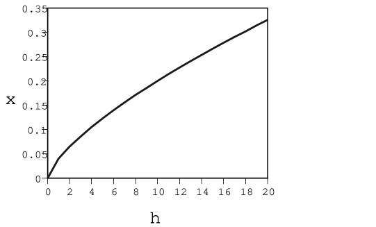
Figure 1: An illustration of the expectation value $x$ as a function of the background field $h$.

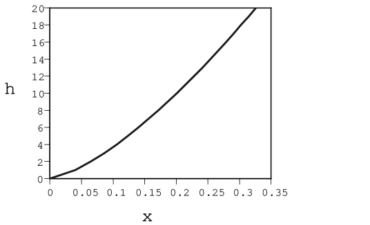
Figure 2: Exchanging $x$ and $h$ in Fig.1, we obtain $h=f^{\prime}(x)$ as a function of $x$.

From the relation

$$h=\left.\displaystyle\frac{df(x)}{dx}\right|_{x=\bar{x}},$$ (27)

we have $df(x)/dx$ as a function of $x$. That is, fitting $h$ by an appropriate function of ${\bar{x}}$, we obtain the functional form of $df(x)/dx$. By integrating this over $x$,

$$\int^{x}_{0}\frac{df(x^{\prime})}{dx^{\prime}}dx^{\prime}=f(x),$$ (28)

we find $f(x)$. In this way, we obtain the topological charge distribution at $\theta=0$.

We should note that this inversion approach is applicable only when $x(h)$ is a monotonic function of $h$. Otherwise, the inverted function $h(x)$ is multivalued. We do not treat this case in the present paper.

At $\theta=0$, the function $f(x)$ is usually directly evaluated through numerical simulation of the topological charge distribution. By contrast, $f(x)$ is determined in the method proposed by Azcoiti et al. as an implicit function through the process represented by (23) through (28). Thus, the $x$-$h$ relation is given by (26). This implies that the functional form of $h(x)$ is obtained numerically. The relation $h(x)=df(x)/dx$ leads to $f(x)$ after integration over $x$.

2.2 Qualitative difference between strong and weak coupling behavior

In a previous paper[4], $P(Q)$ of the two-dimensional CP² model is numerically obtained. Now we study the results from the point of view of the imaginary theta approach. In the strong coupling region ($\beta=$ small $\mathrel{\hbox{\raise 0.86108pt\hbox{$<$}\kern-7.5pt\raise-3.87495pt\hbox{$\sim$}}}1$), $P(Q)$ is approximately given by the Gaussian form

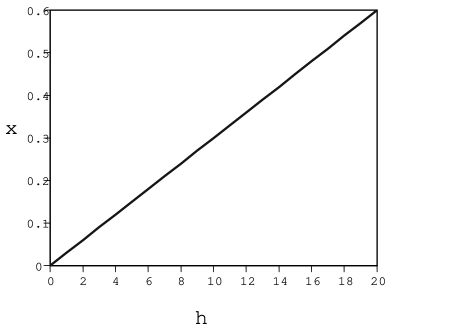
Figure 3: Strong coupling case $x$ as a function of $h$.

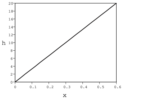
Figure 4: Exchange of $x$ and $h$ in Fig. 3.

$$P(Q)=e^{-\frac{\alpha}{V}Q^{2}}=e^{-V\alpha x_{Q}^{2}},$$ (29)

and

$$f(x)=\alpha x^{2}.$$ (30)

In this case, we have

$$h=f^{\prime}(x)=2\alpha x.$$ (31)

Hence, a linear relation between ($h$ and ${\bar{x}}$) is expected.

In the weak coupling region, the ${\bar{x}}$-$h$ relation is expected to exhibit “step-like behavior”(Fig. 5). In order to make it easy to understand why Fig. 5 is expected, we consider typical simplified behavior of the $Q$ dependence in the weak coupling region[4], with the exponent of $P(Q)$ assumed to be proportional to $|Q|$:

$$P(Q)\sim c^{|Q|}=e^{|Q|\ln c}=e^{-|Q|\ln(1/c)}=e^{-V|x_{Q}|\ln(1/c)}.$$ (32)

The parameter $c$ is known to be quite small from phenomenological considerations. Thus, in this case, we have $f(x)=|x|\ln(1/c)$[4], which we call the “linear $x$ model” hereafter. Then the relation $h=f^{\prime}(x)$ is given by

$$h=f^{\prime}(x)=\left\{\begin{array}[]{rl}\ln(1/c)&=h_{0},\quad x\geq 0,\\ -\ln(1/c)&=-h_{0},\quad x<0.\end{array}\right.$$ (35)

The behavior in the $x\geq 0$ region is shown in Fig. 6. Then, interchanging ${\bar{x}}$ and $h$, we obtain the $h$-${\bar{x}}$ relation, shown in Fig. 5. From Eq.(35), Fig. 6 is obtained first. But from the actual numerical simulation, ${\bar{x}}$ as a function of the background $h$ is computed first. Thus, Fig. 5 is put before Fig. 6.

We set $f_{\rm eff}(x)=f(x)-hx$. By employing the simplified functional form “linear $x$ model”, $f(x)=|x|h_{0}$, we investigate the three cases (i) $-$ (iii) below.

• $0<h<h_{0}$ case:

  We have

  $$f_{\rm eff}(x)=\left\{\begin{array}[]{l}-(h_{0}+h)x,\quad x<0,\\ (h_{0}-h)x,\quad x>0.\end{array}\right.$$ (38)

  Then $\exp(-Vf_{\rm eff}(x))$ is peaked at $x=0$, and we expect ${\bar{x}}\sim 0$.

• $h=h_{0}>0$ case:

  In this case, we have

  $$f_{\rm eff}(x)=\left\{\begin{array}[]{r}-2h_{0}x,\quad x<0,\\ \quad\ 0,\quad x>0.\end{array}\right.$$ (41)

  Then $\exp(-Vf_{\rm eff}(x))$ is constant in the $x>0$ region, and we expect $\bar{x}$ will take a positive value between 0 and the maximum possible value; that is, $\bar{x}$ is undetermined.

• $h>h_{0}>0$ case:

  Here we have

  $$f_{\rm eff}(x)=\left\{\begin{array}[]{l}-(h_{0}+h)x,\quad x<0,\\ -(h-h_{0})x,\quad x>0,\end{array}\right.$$ (44)

  where $h-h_{0}$ is positive. Then $\exp(-Vf_{\rm eff}(x))$ favors as large a value of $x$ as possible and we expect that $\bar{x}$ is given approximately by the maximum possible value. Since $Q$ is bounded from above in the finite volume case, we have $\bar{x}\mathrel{\hbox{\raise 0.86108pt\hbox{$<$}\kern-7.5pt\raise-3.87495pt\hbox{$\sim$}}}Q_{\rm max}/V$. With periodic boundary conditions, $|Q|\mathrel{\hbox{\raise 0.86108pt\hbox{$<$}\kern-7.5pt\raise-3.87495pt\hbox{$\sim$}}}\frac{V}{2}$ is the limit.[1] Then $|x_{Q}|$ is bounded from above by $x_{0}\ (\mathrel{\hbox{\raise 0.86108pt\hbox{$<$}\kern-7.5pt\raise-3.87495pt\hbox{$\sim$}}}1/2)$.

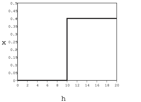
Figure 5: Weak coupling case. The $x$-$h$ relation is inferred from Fig. 6. A step-like increase at $h=h_{0}$ is expected. The value $h_{0}$ is tentatively taken to be 10.0 here.

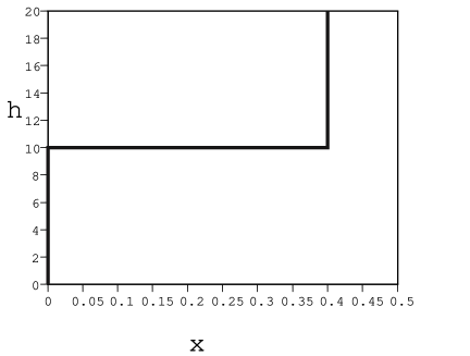
Figure 6: A simplified model in which $f(x)=|x|\ln(1/c)$ gives $h=h_{0}=\ln(1/c)\sim 10.0$ for $x>0$.

Summarizing (i) $-$ (iii), we have found the qualitative behavior of $x$ in the weak coupling region as shown in Fig.5, namely, “step-like behavior” of $\bar{x}$ as a function of the background $h$.

The expectation value ${\bar{x}}$ is expected to be quite small in $0\leq h<h_{0}$ region, while ${\bar{x}}$ becomes approximately $x_{0}$ in the $h>h_{0}$ region. The position of the step-like increase of ${\bar{x}}$ is expected to be located at $h=h_{0}=\ln(1/c)$.

We now give a short comment. In the analysis of finite density QCD, the chemical potential $\mu$ and the nucleon density $n\ (=N/V)$ (where $N$ and $V$ denote the nucleon number and the volume of the system) enter in place of the parameter $h$ and the topological charge density $x$. The low temperature, $T\sim 0$, regime of QCD corresponds to the weak coupling, large $\beta$, regime in the CP^N-1 model, where the topological charge excitation is suppressed due to the fact that only a small fluctuation of the gauge field is allowed. The step-like behavior schematically shown in Fig. 5 is expected to occur in finite density QCD analysis in $T\sim 0$.[10]^,

3 Numerical calculation of the CP² model

3.1 Numerical results

• As described in §2, the expectation value ${\bar{x}}(h)$ was obtained by numerical simulation. The expectation values ${\bar{x}}(h)$ were calculated at various values of the background source points $h$.

• The saddle point method gives the relation

  $$h=f^{\prime}({\bar{x}}).$$ (45)

The above (1) and (2) give the relation between ${\bar{x}}(h)$ and $h$ at many points. From this $x$-$h$ relation, the form of $f^{\prime}({\bar{x}})$ as a function of $\bar{x}$ is obtained by fitting the calculated points. Once the functional form $f^{\prime}(\xi)$ is obtained from this fitting process, we obtain $f(x)$ itself by integrating $f^{\prime}(\xi)$,

$$f(x)=\int^{x}_{0}f^{\prime}(\xi)d\xi.$$ (46)

In Ref. rf:IKY, we discussed the “direct method” and the “indirect method”. The latter is equivalent to the fitting method. The imaginary theta method is simply a candidate for the “indirect method”.

Now we present the results of the numerical simulation of the CP² model using the imaginary theta method. For each $\beta$ and $h$, the number of measurements was set to $10^{5}$.

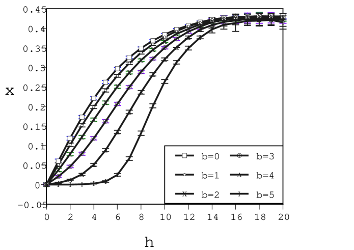
Figure 7: Expectation value $x$ for various values of the background $h$. The values of the inverse coupling $\beta$ are 0.0, 1.0, 2.0, 3.0, 4.0 and 5.0. The lattice size is $L=50$ in all cases.

Figure 7 displays the expectation value $\bar{x}$ with the volume $V=L^{2}\ (L=50)$ for various values of $h=-{\rm Im}\theta$ at $\beta=0.0,1.0,2.0,3.0,4.0$ and $5.0$. In the strong coupling cases ($\beta=0.0,1.0)$, $\bar{x}$ increases linearly as a function of $h$ from the origin:

$${\bar{x}}\sim\frac{1}{2\alpha}h.\quad(h=0.0\sim 5.0)$$ (47)

For much larger values of $h$, $\bar{x}$ exhibits convergence due to the restriction that the topological charge cannot exceed $V/2$ in a finite volume[1]. Thus ${\bar{x}}$ is bounded from above:

$${\bar{x}}<x_{0}\mathrel{\hbox{\raise 0.86108pt\hbox{$<$}\kern-7.5pt\raise-3.87495pt\hbox{$\sim$}}}\frac{1}{2}.$$ (48)

$\underline{\hbox{ Step-like behavior }}$ is observed in the weak coupling regions. In weak coupling cases ($\beta\mathrel{\hbox{\raise 0.86108pt\hbox{$>$}\kern-7.5pt\raise-3.87495pt\hbox{$\sim$}}}5.0$), ${\bar{x}}$ is strongly suppressed in comparison with the strong coupling cases in the region of small $h$ ($h\mathrel{\hbox{\raise 0.86108pt\hbox{$<$}\kern-7.5pt\raise-3.87495pt\hbox{$\sim$}}}5.0)$,

$${\bar{x}}_{\rm weak}\ll{\bar{x}}_{\rm strong}.$$ (49)

In regions of larger $h$, $\bar{x}$ begins to increase rapidly and reaches ${\bar{x}}\sim x_{0}/2$ at $h\sim h_{0}(\beta)$. In $h>h_{0}(\beta)$ region, $\bar{x}$ begins to converge to a constant due to the restriction ${\bar{x}}<x_{0}.$

The position $h_{0}$ of the step-like increase depends on the coupling constant; that is, $h_{0}$ is a function of $\beta$. The observed step-like behavior is not as sharp as the simple sharp step-like increase mentioned in §2 (Fig. 5), but it is clearly observed. For $\beta=5.0$, for example, we have

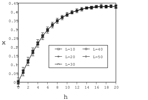
Figure 8: Expectation value $x$ in the strong coupling case ($\beta=0.0$). Lattice sizes are $L=$10, 20, 30, 40 and 50.

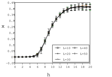
Figure 9: Expectation value $x$ for various values of $h$ in the weak coupling case ($\beta=5.0$). Lattice sizes are $L=$10, 20, 30, 40 and 50.

$$\begin{array}[]{rl}&h_{0}=\ln(1/c)\sim 10.0.\end{array}$$ (51)

Note that all $\bar{x}$ in Fig. 7 are monotonic functions of $h$.

Figure 8 displays $\bar{x}$ in the strong coupling case ($\beta=0$) for various sizes, $L=10,20,30,40$ and $50$. The values of $\bar{x}$ for different sizes coincide and exhibit linear dependence on $h$. Because $h=f^{\prime}(x)$, a linear dependence of $\bar{x}$ on $h$ for $h\mathrel{\hbox{\raise 0.86108pt\hbox{$<$}\kern-7.5pt\raise-3.87495pt\hbox{$\sim$}}}5.0$, i.e.,

$${\bar{x}}=\frac{1}{2\alpha}h,$$ (52)

gives

$$f^{\prime}(x)=2\alpha x.$$ (53)

Integrating this, we obtain

$$f(x)=\alpha x^{2},$$ (54)

namely a Gaussian distribution for $P(Q)$:

$$P(Q)\propto\exp(-Vf(x))=\exp(-\frac{\alpha}{V}Q^{2}).$$ (55)

Figure 9 displays $\bar{x}$ in the weak coupling case ($\beta=5.0$) for various sizes, $L=10,20,30,40$ and $50$. Smooth step-like behavior is found for all these sizes. More detailed behavior for small $h$ is shown in Fig. 10. For small $h$, some dependence on the value of $L$ is observed. The global behavior for the values $h=0.0$ - 20.0, however, is almost the same for all values of $L$ considered here(Fig. 9).

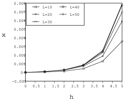
Figure 10: Expectation value of $\bar{x}$ in the weak coupling case ($\beta=5.0$) at smaller $h\ (0.0\sim 5.0)$. The lattice size dependence is clear for smaller $L\ (10$ - 30). The lattice size dependence is weaker for $L=$ 40 and 50.

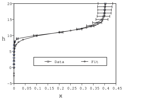
Figure 11: Expectation value of $h=f^{\prime}(x)$ as a function of $x$ for weak coupling ($\beta=6.0$) at $L=$ 50. Both experimental data and a fit [Eq. (72)] are shown.

In Fig. 11, $h$ vs $\bar{x}$ in the case of weak coupling, $\beta=6.0$, for $L=50$ is shown. Plateau-like behavior of $h$ at $h=h_{0}\sim 11.0$ is clearly seen. It is smoother than that in the simple case considered in the previous section, but Fig. 11 is the reminiscent of the plateau-like behavior (Fig. 6). To see the detailed behavior for values of $h$ near the origin, a log-log plot is shown in Fig. 12.

3.2 Real $\theta$, imaginary $\theta$ and analytic continuation

Employing a simple “linear $x$ model”, we now investigate the role of the imaginary theta method. The linear $x$ model is defined by

$$f(x)=|x|h_{0},\qquad h_{0}=\ln(1/c)>0.$$

Hence, the exponent $f(x)$ of the topological charge distribution is a linear function of the topological charge (divided by the volume). In the case of real $\theta$, we have

$$Z_{V}(\theta)= \sum_{x_{n}}e^{-Vf(x_{n})}e^{iV\theta x_{n}}$$ (56)

$$= \sum_{x_{n}}e^{-V|x_{n}|h_{0}}e^{iV\theta x_{n}}.$$ (57)

In the case of imaginary $\theta$, $\theta=-ih$ is inserted, and we have

$$Z_{V}(h) = \sum_{x_{n}}e^{-V|x_{n}|h_{0}}e^{Vx_{n}h}\qquad$$ (58)

$$= ({\rm negative}\ Q)+(Q=0)+({\rm positive}\ Q)$$ (59)

$$= \sum_{n=1}^{N}e^{-h_{0}n-hn}+1+\sum_{n=1}^{N}e^{-h_{0}n+hn}$$ (60)

$$= \sum_{n=1}^{N}t^{n}+1+\sum_{n=1}^{N}s^{n},$$ (61)

where $x_{n}=n/V=Q/V$, $s=e^{-h_{0}+h}$ and $t=e^{-h_{0}-h}$, and the finite volume imposes an upper bound of the topological charge $Q$ at $N$.

Then the partition function is given by

$$Z_{V}(h)=\frac{t-t^{(N+1)}}{1-t}+1+\frac{s-s^{(N+1)}}{1-s}.$$ (62)

In the case of real $\theta$, $s(\theta)=e^{-h_{0}}e^{i\theta}$ and $t(\theta)=e^{-h_{0}}e^{-i\theta}$ lead to $|s(\theta)|<1$ and $|t(\theta)|<1$. Thus, $s^{N+1}$ and $t^{N+1}$ approach zero, and Eq. (62) becomes

$$Z_{V}(\theta) \sim \frac{t(\theta)}{1-t(\theta)}+1+\frac{s(\theta)}{1-s(\theta)}$$ (63)

$$= \frac{1-c^{2}}{1-2c\cos\theta+c^{2}},$$ (64)

where $c=e^{-h_{0}}\ll 1$.

In order to address the question of whether it is possible to extend real $\theta$ to imaginary $\theta$, let us study the following two cases.

• Imaginary $\theta$: $\theta=-ih$, with $|h|<h_{0}$

  In this case, $s=e^{-h_{0}+h}<1$ and $t=e^{-h_{0}-h}<1$, and both $s^{N+1}$ and $t^{N+1}$ can be safely ignored. Then we obtain

  $$Z_{V}(h)\to\frac{t}{1-t}+1+\frac{s}{1-s}$$ (65)

  $$=\frac{1-c^{2}}{1-2c\cosh h+c^{2}}.$$ (66)

  Equation (66) is then simply analytically continued to Eq.(64) by taking $h\to i\theta$.

• Imaginary $\theta$: $\theta=-ih$, with $|h|>h_{0}$

  We consider $h>h_{0}>0.$ It should be noted that

  $$t=e^{-h_{0}-h}<1,\qquad s=e^{-h_{0}+h}>1.$$ (67)

  In this case, $s$ is greater than unity. Thus, the leading contribution to $Z_{V}(h)$ is given by

  $$Z_{V}(h)\sim\frac{-s^{N+1}}{1-s}.$$ (68)

  From Eq. (68), the expectation value of $x$ is

  $${\bar{x}}=\frac{1}{V}\frac{dZ/dh}{Z}\sim\frac{N}{V}={\rm finite}=x_{0}\mathrel{\hbox{\raise 0.86108pt\hbox{$<$}\kern-7.5pt\raise-3.87495pt\hbox{$\sim$}}}1/2.$$ (69)

  An important point is that $Z_{V}(h)$ is not simply obtained in the $h>h_{0}$ region by analytic continuation from Eq. (64) by taking $\theta\to-ih$. Rather, $Z_{V}(h)$ is given by Eq. (68), which is completely different from the analytic continuation form Eq. (66) in the $h>h_{0}$ region.

This simple “linear $x$ model” provides the important lesson that there is a case in which imaginary $\theta$ does not yield the real $\theta$ result by analytic continuation. Rather, the imaginary $\theta$ method is used as a fitting procedure for the topological charge distribution $P(Q)$ at $\theta=0$.[7]

In the weak coupling region, ${\bar{x}}$ exhibits step-like behavior as a function of $h$. For $h\mathrel{\hbox{\raise 0.86108pt\hbox{$<$}\kern-7.5pt\raise-3.87495pt\hbox{$\sim$}}}h_{0}=\ln(1/c)$, ${\bar{x}}$ is close to zero. Then, it increases suddenly at $h\sim h_{0}$ and then satisfies ${\bar{x}}\sim x_{0}$ for $h\mathrel{\hbox{\raise 0.86108pt\hbox{$>$}\kern-7.5pt\raise-3.87495pt\hbox{$\sim$}}}h_{0}$. Actually, the $h$-${\bar{x}}$ relation obtained numerically does not exhibit an abrupt step-like increase at $h\sim h_{0}$, but a somewhat gentle one. Simple functional form representing this “gentle” step-like behavior is expressed as a function of $h$ as

$$x=\frac{x_{0}e^{c_{e}(h-h_{0})}}{1+e^{c_{e}(h-h_{0})}},$$ (70)

where ${\bar{x}}$ is written as $x$. The parameter values are

$$h_{0}\sim 11.0,\ x_{0}\sim 0.4031,\ c_{e}\sim 0.95$$

for $\beta=6.0$ and $L=50$.

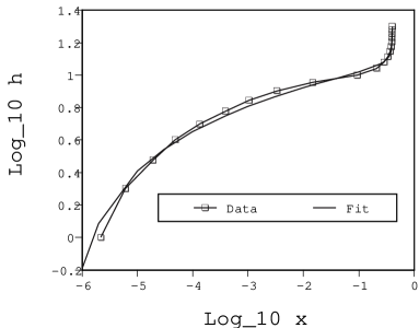
Figure 12: In order to see the detailed behavior of Fig. 11 for smaller $h$, a log-log plot is shown for the same set of numerical data as in Fig. 11.

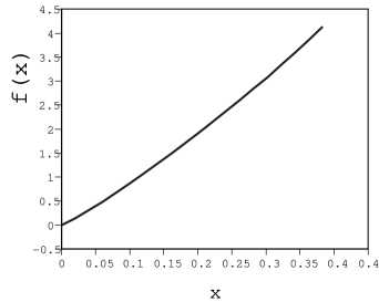
Figure 13: Integrating Eq. (72), we obtain the analytical form $f(x)$ [Eq. (74)] for this case.

This relation is easily inverted. We have

$$e^{c_{e}(h-h_{0})}=\frac{x}{x_{0}-x}$$ (71)

and

$$h=h_{0}+\frac{1}{c_{e}}\{\ln x-\ln(x_{0}-x)\}.$$ (72)

Since $h$ is given by $h=f^{\prime}(x)$, we integrate Eq. (72) and obtain

$$f(x) = \int^{x}f^{\prime}(x^{\prime})dx^{\prime}=\int^{x}h(x^{\prime})dx^{\prime}\qquad$$ (73)

$$= h_{0}x+\frac{1}{c_{e}}\{x\ln x+(x_{0}-x)\ln(x_{0}-x)\}+d,$$ (74)

where $d$ is an integration constant. If we assume $f(0)=0$, $d$ becomes

$$d=\frac{-1}{c_{e}}x_{0}\ln x_{0}.$$ (75)

The value of $h$ for $\beta=6.0$ and $L=50$ is plotted as a function of $x={\bar{x}}$ in Fig. 11 and 12. In these figures, the fitting function given in Eq. (72) is also shown. The integrated $f(x)$ is plotted as a function of $x$ in Fig. 13. An almost linear dependence of $f(x)$ on $x$ is observed in the weak coupling region.

4 Conclusions and discussion

The inversion approach[7] based on the imaginary theta method[6] was investigated in both strong and weak coupling regions. In the strong coupling region, the expectation value ${\bar{x}}$ exhibits linear dependence on $h$ for $h\mathrel{\hbox{\raise 0.86108pt\hbox{$<$}\kern-7.5pt\raise-3.87495pt\hbox{$\sim$}}}5.0$. In the weak coupling region, ${\bar{x}}$ is much smaller than that in the strong coupling region:

$${\bar{x}}({\rm weak})\ll{\bar{x}}({\rm strong})\quad{\rm for}\ h\mathrel{\hbox{\raise 0.86108pt\hbox{$<$}\kern-7.5pt\raise-3.87495pt\hbox{$\sim$}}}5.0.$$ (76)

The expectation value ${\bar{x}}$ is expected to be quite small in the region $0\leq h<h_{0}$, while ${\bar{x}}$ is approximately equal to $x_{0}$ in the region $h>h_{0}$. The position of the step-like increase of ${\bar{x}}$ is expected to be located at $h=h_{0}=\ln(1/c)$.

The expectation value ${\bar{x}}$ thus displays a step-like increase at $h\sim h_{0}=\ln(1/c)\sim 10.0\sim 11.0$. The parameter $c$ represents the probability of a single topological charge excitation in the weak coupling region. The value of $c$ is quite small.

We have numerically calculated ${\bar{x}}$ for each $h$, thus obtaining ${\bar{x}}$ as a function of $h$. Then we have obtained $h$ as a function of ${\bar{x}}$ by inverting ${\bar{x}}$ and $h$. In the large $V$ limit, $h$ is identified with $f^{\prime}(x)$, and ${\bar{x}}$ is simply written as $x$. If we fit $h$ with an appropriate functional form $h_{\rm fit}(x)$, then $f(x)$ is obtained by integrating $h_{\rm fit}(x)$ as

$$f(x)=\int^{x}f^{\prime}(x^{\prime})dx^{\prime}=\int^{x}h_{\rm fit}(x^{\prime})dx^{\prime},$$ (77)

where $f(x)$ denotes $f(x)=-V^{-1}\ln P(Q)$. In this way $f(x)$, namely, $P(Q)$ at $\theta=0$, is obtained.

This process shows that the inversion approach in the imaginary theta method is not the analytic continuation from $h$ to non-zero theta, but $P(Q)$ at $\theta=0$ is obtained as one of the products of this approach. A simplified fitting function $h_{\rm fit}(x)$ is presented in §3, and the result, $f(x)$, is given for that fitting function. The obtained function $f(x)$ [see Eq. (77)] is shown in Fig. 13.

The purpose of the present paper is to clarify the meaning of the inversion approach proposed by Azcoiti et al. For this purpose, we have chosen a simple model, the CP² model. In our previous analysis[4], it was shown that this model exhibits qualitatively different behavior of $P(Q)$ in the strong and weak coupling regions. This difference emerges as that in the ${\bar{x}}$-$h$ relation of the imaginary theta method. Since we have employed the standard action, and this model is contaminated by dislocations, precise information about continuum physics cannot be obtained. Although a further investigation of the continuum limit is left for a future study, what we have clarified here, i.e., that the ${\bar{x}}$-$h$ relation in the weak coupling region exhibits step-like behavior, should not be altered if a more realistic model were employed. For example, in our previous analysis [13] of the CP³ model with a fixed-point action, it is shown that the topological quantities, such as $P(Q)$ and the expectation value $\langle Q\rangle_{\theta}$, exhibit nice scaling behavior, and that $P(Q)$ behaves differently in the strong and weak coupling regions. Specifically, we studied the behavior of the effective exponent of $P(Q)$, $\gamma_{\rm eff}$, and we found that $\gamma_{\rm eff}$ in the weak coupling region is smaller than that in the strong coupling region (Gaussian). This suggests the possibility of step-like behavior of ${\bar{x}}$-$h$ in the continuum limit. Further study of this point is needed.

“The step-like increase” of ${\bar{x}}$ at $h\sim h_{0}$ in the weak coupling region ($1/\beta\sim 0$) is shematically shown in Fig. 5. The results of the actual numerical simulation are shown in Fig. 9. As stated at the end of §2, the $h$-$\bar{x}$ relation is quite similar to the $\mu$-$n$ (chemical potential vs nucleon density) relation in QCD. For $T\sim 0$ (where $T$ denotes temperature), a step-like increase at $\mu\sim\mu_{0}$ is expected, as shown in Figure 8-10(a) of the textbook of Kogut and Stephanov.[10] Further investigation of the correspondence between $h$-$\bar{x}$ in the CP^N-1 and $\mu$-$n$ relation in QCD is an interesting problem.