Excited hadrons on the lattice: Mesons

Abstract

We present results for masses of excited mesons from quenched calculations using chirally improved quarks at pion masses down to 350 MeV. The key features of our analysis are the use of a matrix of correlators from various source and sink operators and a basis which includes quark sources with different spatial widths, thereby improving overlap with states exhibiting radial excitations.

I Introduction

Ground-state hadron spectroscopy has been at the forefront of the studies performed by the lattice QCD community. The exponential decay behavior of the mass eigenstate contributions to Euclidean-time correlators makes extraction of the lightest state straightforward: at large time separations, the ground-state mass naturally dominates the correlator, which then displays a single exponential in time. Excited states, however, appear as subleading exponentials, which in practice are rather difficult to separate, not only from the ground-state contribution, but also from those due to other excited states.

A few methods are currently in use to deal with this problem. A straightforward fit to a finite sum of exponentials is sometimes possible, usually when high statistics are available. Constrained fitting constrainedfits and the Maximum Entropy Method maximumentropy are also options, but these, like the first method, can encounter problems when faced with states which lie close in mass, or when unphysical contributions appear due to quenching (ghosts).

We employ a different method, one based upon the variational method devised by Michael Mi85 , and later elaborated by Lüscher and Wolff LuWo90 . The distinguishing characteristic of our approach is the use of several hadron interpolators which contain quark wavefunctions covariantly smeared to approximate Gaussians of different widths BuGaGl04 . Using such a basis of source and sink operators, it is our plan to improve overlap with physical states which may involve a radial excitation. In a recent paper BuGaGl05 , it has been demonstrated that this method also clearly separates ghost contributions.

In the present work, we describe the method in detail and report results for the meson sector. Another paper will contain our latest results for baryons.

II The method

Our calculation is based upon the variational method Mi85 ; LuWo90 . The central idea is to use several different interpolators $O_{i},i=1,\ldots\,N$ with the quantum numbers of the desired state and to compute all cross correlations

$$C(t)_{ij}\;=\;\langle\,O_{i}(t)\,\overline{O}_{j}(0)\,\rangle\;.$$ (1)

In Hilbert space these correlators have the decomposition

$$C(t)_{ij}\;=\;\sum_{n}\langle\,0\,|\,O_{i}\,|\,n\,\rangle\langle\,n\,|\,O_{j}^{\dagger}\,|\,0\,\rangle\,e^{-t\,M_{n}}\;.$$ (2)

Using the factorization of the amplitudes one can show LuWo90 that the eigenvalues $\lambda^{(k)}(t)$ of the generalized eigenvalue problem

$$C(t)\,\vec{v}^{(k)}\;\;=\;\;\lambda^{(k)}(t)\,C(t_{0})\,\vec{v}^{(k)}\;,$$ (3)

behave as

$$\lambda^{(k)}(t)\;\propto\;e^{-t\,M_{k}}\,[\,1+{\cal O}(e^{-t\,\Delta M_{k}})\,]\;,$$ (4)

where $M_{k}$ is the mass of the $k$-th state and $\Delta M_{k}$ is the difference to the mass closest to $M_{k}$ WeMo06 . In Eq. (3) the eigenvalue problem is normalized with respect to a timeslice $t_{0}<t$.

Equation (4) shows that the eigenvalues each decay with their own mass: The largest eigenvalue decays with the mass of the ground state, the second largest eigenvalue with the mass of the first excited state, etc. Thus, the variational method allows one to decompose the signal into those for ground and excited states, as well as ghost contributions BuGaGl05 , and therefore, simple, stable two-parameter fits become possible.

We remark that also for the regular eigenvalue problem,

$$C(t)\,\vec{v}^{(k)}\;\;=\;\;\lambda^{(k)}(t)\,\vec{v}^{(k)}\;,$$ (5)

a behavior of the type (4) can be shown LuWo90 . We find that in a practical implementation with our sources the results and the quality of the data are essentially unchanged whether we use the regular or the generalized eigenvalue problem.

The key to a successful application of the variational method is the choice of the basis interpolators. They should be linearly independent, and as orthogonal as possible, while at the same time, able to represent the physical state as well as possible. Furthermore, they should be numerically cheap to implement.

For meson spectroscopy it is well known that different Dirac structures can be used to construct interpolators with the quantum numbers one is interested in. In this paper we consider interpolators of the form

$$O\;=\;\overline{\psi}^{(f_{1})}\,\Gamma\,\psi^{(f_{2})}\;,$$ (6)

where $f_{i}$ are flavor labels. We use matrix/vector notation for Dirac and color indices and $\Gamma$ is an element of the Clifford algebra. Depending on what combination of gamma-matrices one uses for $\Gamma$, the interpolator $O$ will have different quantum numbers. We list these in Table 1.

Table 1: Quantum numbers of the interpolators (6) for different choices of $\Gamma$. We remark that the classification with respect to $C$ is for flavor degenerate interpolators only.

state	$J^{PC}$	$\Gamma$	particles
scalar	$0^{++}$	$\mathds{1}$	$a_{0}$
pseudoscalar	$0^{-+}$	$\gamma_{5}\,,\,\gamma_{4}\gamma_{5}$	$\pi,K$
vector	$1^{--}$	$\gamma_{i}\,,\,\gamma_{4}\gamma_{i}$	$\rho,K^{*},\phi$
pseudovector	$1^{++}$	$\gamma_{i}\gamma_{5}$	$a_{1}$
pseudovector	$1^{+-}$	$\gamma_{i}\gamma_{j}$	$b_{1}$

However, it is well known (see, e.g., blumetal ; BrCrGa04 ) that correlating operators with different Dirac structures alone does not provide a sufficient basis to obtain good overlap with excited states. For many excited hadrons the spatial wavefunctions are expected to have nodes. In BuGaGl04 ; BuGaGl04b it was proposed, and tested on small lattices, to use Jacobi smeared quark sources of different widths to allow for nodes in the radial wavefunction. Other lattice efforts Al93 ; LHP05 have also seen the need of using spatially extended operators.

In a lattice spectroscopy calculation the hadron correlators are built from quark propagators $D^{-1}$ acting on a source $s$,

$$\sum_{\vec{y},\rho,c}D^{-1}(\vec{x},t\mid\vec{y},0)_{\beta\,\rho\atop b\,c}\;s^{(\alpha,a)}(\vec{y},0)_{\rho\atop c}\;.$$ (7)

If the source is point-like, i.e., $s=s_{0}$, with

$$s^{(\alpha,a)}_{0}(\vec{y},0)_{\rho\atop c}\;\;=\;\;\delta(\vec{y},\vec{0})\;\delta_{\rho\,\alpha}\;\delta_{c\,a}\;,$$ (8)

then the two quarks in (6) both sit on the same lattice site. Certainly this is not a very physical assumption.

The idea of Jacobi smearing jacobi1 ; jacobi2 is to create an extended source by iteratively applying the hopping part of the Wilson term within the timeslice of the source:

$$s^{(\alpha,a)} = M\;s_{0}^{(\alpha,a)}\;\;\;,\;\;\;\;M\,=\,\sum_{n=0}^{N}\,\kappa^{n}\,H^{n}\;,$$

$$H(\vec{x},\vec{y}\,) = \sum_{j=1}^{3}\Big{[}\,U_{j}(\vec{x},0)\,\delta(\vec{x}+\hat{j\,},\vec{y}\,)$$ (9)

$$\qquad+\;\,U_{j}(\vec{x}\!-\!\hat{j\,},0)^{\dagger}\,\delta(\vec{x}-\hat{j\,},\vec{y}\,)\,\Big{]}\;.$$

Applying the inverse Dirac operator as shown in (7) connects the source at timeslice $t=0$ to the lattice points at timeslice $t$. There an extended sink may be created by again applying the smearing operator $M$.

Jacobi smearing has two free parameters, the hopping parameter $\kappa$ and the number of smearing steps $N$. They can be used to create sources and sinks with approximately Gaussian profiles of different widths. In Fig. 1 we show two such profiles $P(r)$ as a function of the radius $r$. For mapping these profiles we use the definition

$$P(r)\;=\;\sum_{\vec{y}}\delta\Big{(}\,|\vec{y}\,|-r\,\Big{)}\,\sum_{b}\,\Big{|}s^{(\alpha,a)}(\vec{y},0)_{\alpha\atop b}\Big{|}\;.$$ (10)

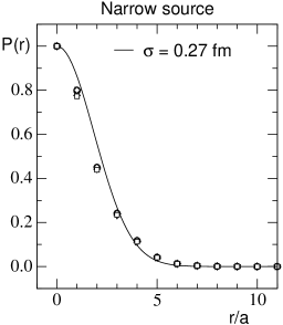
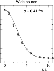
Figure 1: Profiles $P(r)$ of the narrow and wide source as a function of the radius $r$ (for the $\beta=7.90$ lattice). The symbols are our data points. The curves are the target Gaussian distributions (with half width $\sigma$) which we approximate by the profiles $P(r)$.

Table 2: Parameters of our simulation. We list the lattice size, the inverse coupling $\beta$, the number of configurations, the lattice spacing $a$, the cutoff $a^{-1}$, and the smearing parameters $N$ and $\kappa$ for the narrow and wide sources.

size	$\beta$	confs.	$a$[fm]	$a^{\!-1}$[MeV]	$N\,(n,w)$	$\kappa\,(n,w)$
$20^{3}\!\times\!32$	8.15	100	0.119	1680	22, 62	0.21, 0.1865
$16^{3}\!\times\!32$	7.90	100	0.148	1350	18, 41	0.21, 0.1910

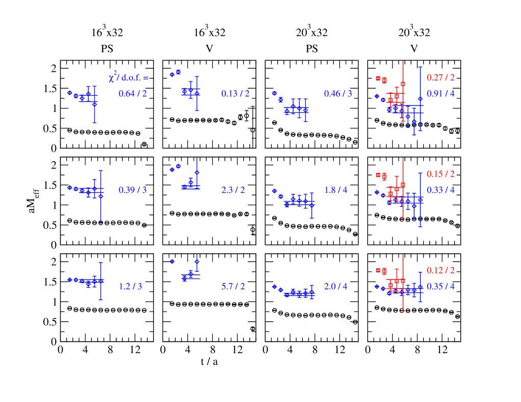
Figure 2: Effective mass plots for pseudoscalar (PS) and vector (V) mesons from our coarse ($16^{3}\times 32$, $a=0.148$ fm, with $am_{q}=0.05,0.1,0.2$ from top to bottom) and fine ($20^{3}\times 32$, $a=0.119$ fm, with $am_{q}=0.04,0.08,0.16$) lattices. Both ground and excited states are shown, along with the $M\pm\sigma_{M}$ results (horizontal lines) from correlated fits to the corresponding time intervals. The numbers in the plots are the $\chi^{2}$ per degree of freedom values for the fits to the excited-state plateaus.

The parameters $\kappa$ and $N$ were adjusted such that the narrow source approximates a Gaussian with a half width (i.e., standard deviation) of 0.27 fm and the wide source a Gaussian with a half width of 0.41 fm. The corresponding smearing parameters are listed in Table 2. The values of the smearing parameters are chosen such that simple linear combinations of our two sources allows one to approximate the ground- and first-excited state wavefunctions of the 3-d harmonic oscillator (with a half width of $\sigma=0.33$ fm for the ground state). We stress that we do not impose such linear combinations, but rather use the simple $n$, $w$ sources for the basis interpolators in the variational method and leave it to the simulation to determine the physical superpositions.

The interpolators which we actually consider in our correlation matrix are flavor triplet operators of the form,

$$O^{\Gamma}\;=\;\overline{u}\,\Gamma\,d\;.$$ (11)

This avoids the need to calculate disconnected pieces. For a given Clifford element $\Gamma$ both $\overline{u}$ and $d$ sources can be wide or narrow which gives the 4 possibilities (the subscripts $n,w$ denote the type of smearing used)

$$O^{\Gamma}_{nn}\,=\,\overline{u}_{n}\,\Gamma\,d_{n} \;,\; O^{\Gamma}_{wn}\,=\,\overline{u}_{w}\,\Gamma\,d_{n}\;,$$

$$O^{\Gamma}_{nw}\,=\,\overline{u}_{n}\,\Gamma\,d_{w} \;,\; O^{\Gamma}_{ww}\,=\,\overline{u}_{w}\,\Gamma\,d_{w}\;.$$ (12)

In addition, we have two choices for $\Gamma$ in the vector and pseudoscalar sectors such that for these cases we have a basis of 8 interpolators. For scalars and pseudovectors we restrict ourselves to 4 interpolators.

In the case of degenerate quark masses, $O^{\Gamma}_{wn}$ and $O^{\Gamma}_{nw}$ give rise to identical correlators. This fact reduces the correlation matrices to $6\times 6$ for vector and pseudoscalar states and to $3\times 3$ for scalar and pseudovector states. For the strange mesons, obtained by replacing the down quark in (11) by a strange quark, the degeneracy is lifted and we are free to work with the full $8\times 8$ and $4\times 4$ correlation matrices.

Our quenched study is done with the Lüscher-Weisz gauge action Luweact at two different values of the inverse gauge coupling $\beta$. The lattice spacing $a$ was determined in scale using the Sommer parameter. We use lattices of two different sizes, such that the spatial extent in physical units is kept constant at 2.4 fm. This allows us to compare the results at two different values of the cutoff, $a^{-1}=1680$ MeV and $a^{-1}=1350$ MeV. For the fermions we use the chirally improved Dirac operator chirimp . It is an approximation of a solution of the Ginsparg-Wilson equation GiWi82 , with good chiral behavior bgrlarge . The parameters of our calculation are collected in Table 2. We determine the strange quark mass via interpolations in the heavy-quark mass which match the (light-quark mass extrapolated) pseudoscalar K meson mass to the physical value. (These configurations have also been used in another study GaHuLa05 to determine low energy constants.)

We remark that the CI operator has one term which is next-to-nearest neighbor. This has to be kept in mind when selecting fit ranges for masses. Exactly what is to be considered a safe minimum time separation before fitting is not, however, a simple matter. In the present case, we limit ourselves to values larger than $\Delta t=2$.

III Results

III.1 Effective masses and fit ranges

Since this is a report on lattice spectroscopy, we begin the discussion of our results in the standard manner: with effective masses. Having performed the necessary diagonalizations of the correlator matrices, we determine the effective masses from ratios of eigenvalues on adjacent timeslices:

$$aM_{eff}^{(k)}\,\Big{(}t+\frac{1}{2}\Big{)}\;=\;\ln\left(\frac{\lambda^{(k)}(t)}{\lambda^{(k)}(t+1)}\right)\;.$$ (13)

Errors for such quantities are determined via a single-elimination jackknife procedure.

We note that the quality of the plateaus which we obtain here can depend upon the basis chosen. This is simply due to the fact that the various interpolators have different overlap with the states which contribute to the higher-order corrections in Eq. (4) (e.g., see Ref. Al93 ). An appropriate choice of operator combination (including the possibility of further limiting the basis) can therefore minimize such corrections, improving the plateaus in effective mass (and correspondingly, in the eigenvector components).

In Fig. 2, we present our effective mass plots for what we consider to be our optimal operator combinations ($n\Gamma n$, $n\gamma_{4}\Gamma n$, $n\gamma_{4}\Gamma w$, $w\gamma_{4}\Gamma w$ for pseudoscalar and vector mesons on our coarse lattices; $n\gamma_{4}\Gamma n$, $n\gamma_{4}\Gamma w$, $w\gamma_{4}\Gamma w$ for the same mesons on our fine lattices; and $n\Gamma n$, $n\Gamma w$, $w\Gamma w$ otherwise). Shown are results for the pseudoscalar and vector mesons from three quark masses on both sets of lattices. In each case, the effective masses from the largest two eigenvalues (largest three for the vectors on the fine lattice) are displayed. The horizontal lines in the plots mark the $M\pm\sigma_{M}$ values which arise from correlated fits to the corresponding time intervals (we fit only when we see a plateau of at least three successive effective-mass points). Also given in the plots are the $\chi^{2}/d.o.f.$ values for the fits to the excited-state plateaus. Here, one can see questionable plateaus, and hence poor fits, for the coarse-lattice excited vectors at high quark mass, but this is the only place where such high $\chi^{2}/d.o.f.$ values occur. For all other fits, $\chi^{2}/d.o.f.\lesssim 1$.

To be sure that we are dealing (within statistical errors) with a single mass eigenstate, we check that the corresponding eigenvectors remain constant over the same region where we fit the eigenvalues for the mass. An example of such a test is shown in Fig. 3, where we display the second eigenvector for one of the vector mesons on our fine lattices. It is obvious here that plateaus for this state cannot be trusted before $t=4a$, even though when looking at the corresponding effective masses, one is tempted to start the fit at $t=3a$ (see the right-most column in Fig. 2). We make sure that all our fit ranges obey (within errors) such restrictions. (This procedure accounts for the enlargement of error bars for the aforementioned state since we reported preliminary results for the mesons BuHaHi05 . We are simply being more conservative now.)

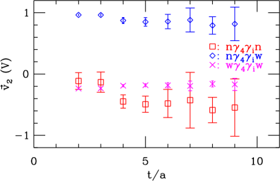
Figure 3: Eigenvector for the first-excited vector meson on our $20^{3}\times 32$ fine lattices ($a\approx 0.12$ fm, $am_{q}=0.06$, $t_{0}=1a$). The eigenvector on each time slice is normalized such that $|\vec{v}|=1$. There is a clear jump in the relative components from $t=3a$ to $t=4a$, a plateau forming afterwards. In this situation, we fit starting at $t=4a$, even though the corresponding effective mass plot shows a plateau starting sooner. We apply similar restrictions to all our fit ranges.

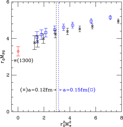
Figure 4: Excited-state pseudoscalar (PS) masses vs. $M_{\pi}^{2}$ for both lattice spacings. The quark masses are degenerate. All quantities are in units of the Sommer parameter, $r_{0}$. The diamond represents the experimental point and the vertical lines mark the values of $r_{0}^{2}M_{\pi}^{2}$ corresponding to the physical strange quark mass.

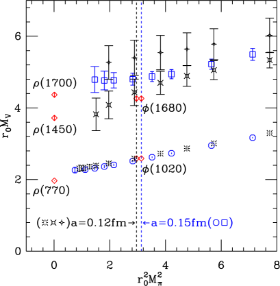
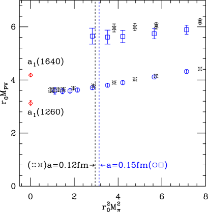
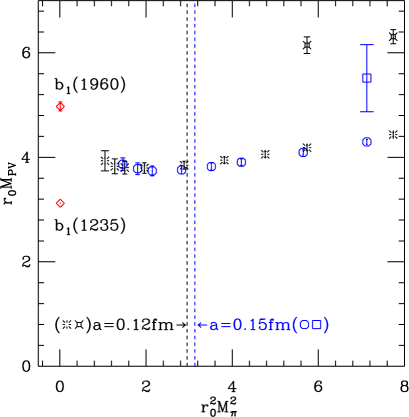
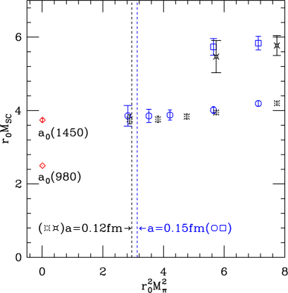
Figure 5: Ground- and excited-state meson masses vs. $M_{\pi}^{2}$ for both lattice spacings. Vector (V), pseudovector (PV), and scalar (SC) mesons appear. The quark masses are degenerate. All quantities are in units of the Sommer parameter, $r_{0}$. The diamonds represent the experimental points and the vertical lines mark the values of $r_{0}^{2}M_{\pi}^{2}$ corresponding to the physical strange quark mass.

III.2 Quark mass dependence

In Figs. 4$-$6, we plot the resulting hadron masses versus the ground-state pseudoscalar mass-squared ($\propto m_{q}$), all in units of the Sommer parameter $r_{0}$. All plots display results from both our coarse and fine lattices. The vertical lines mark the values of $r_{0}^{2}M_{\pi}^{2}$ which arise when we use the strange quark mass in the degenerate-quark-mass pseudoscalar; i.e., these mark the point where the mass of each of the light ($u,d$) quarks in the corresponding meson equals the strange quark mass.

Figure 4 shows the excited pseudoscalar masses. The results from both lattice sets appear consistent with the experimental value and, given the consistency of the two sets (within statistical errors), no large discretization effects are apparent.

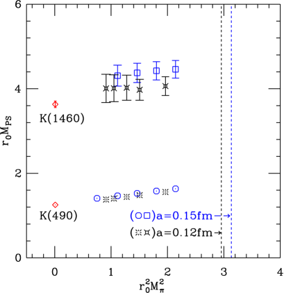
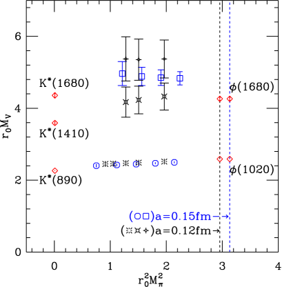
Figure 6: Ground- and excited-state meson masses vs. $M_{\pi}^{2}$ for both lattice spacings. Both pseudoscalar (left) and vector (right) mesons appear. One quark mass is fixed to the physical strange quark mass. All quantities are in units of the Sommer parameter, $r_{0}$. The diamonds represent the experimental points and the vertical lines mark the values of $r_{0}^{2}M_{\pi}^{2}$ corresponding to the physical strange quark mass.

In Fig. 5, we show the ground- and excited-state masses of the vector, pseudovector, and scalar mesons. For the vector mesons on the coarse lattices, only one excited state is extracted (another, slightly lighter effective mass plateau was seen, but since the eigenvectors were not stable over the same region, no fits were performed). This state either corresponds to the $\rho(1700)$ or it suffers apparently significant discretization effects. On the fine lattices, two such excited states are resolved which appear consistent with the physical states; the statistical errors, however, are larger, possibly hiding any residual systematic effects.

The pseudovector and scalar mesons present more difficulties. Fewer effective mass plateaus can be found for excited states; for the $b_{1}$ and scalar mesons, they are virtually non-existent. There are already significant problems for the ground states. At small quark masses, it becomes obvious that the pseudovectors suffer large quenching and/or finite-volume effects, causing an apparent enhancement of the mass.

The upward curvature seen in the ground-state vectors (at least on the coarse lattices) and pseudovectors may be partly explained by quenching effects. Quenched chiral perturbation theory for vector mesons BoChFa96 predicts a negative $M_{\pi}$ term, which could certainly cause the observed enhancement at low quark masses.

For the scalar meson plot similar curvature is seen, and this despite the fact that our method removes the dominant influences of ghosts BuGaGl05 . The entire scalar plot also appears to be shifted vertically, making one wonder whether the ground-state $\bar{u}d$ scalar meson even corresponds to the $a_{0}(980)$. Other lattice studies PrDaIz04 ; SuTsIs05 find that, in fact, it does not.

Our interpolators may be a poor choice of operators for the pseudovector and scalar states. One might achieve better results by altering the $S$-wave nature of our smeared quark wavefunctions. In a future study, we plan to apply covariant derivatives to our smeared sources, providing interpolators which better mimic $P$-wave orbital excitations and, hopefully, improving overlap with the pseudovector and scalar mesons.

In Fig. 6, we present our results for strange-light pseudoscalar and vector mesons. The abscissa is again $r_{0}^{2}M_{\pi}^{2}$, but now this only corresponds to the light-quark mass and we therefore only plot values which are lighter than the strange-quark mass. The general picture here is similar to that seen for the degenerate-quark-mass pseudoscalar and vector mesons: Again, perhaps partly due to somewhat large statistical errors for the excited states, the results for the pseudoscalar mesons appear consistent with the experimental values. The same also applies to the vector mesons on the fine lattices, while the coarse-lattice excited vector results appear systematically high.

III.3 Comparison with results on smaller lattices

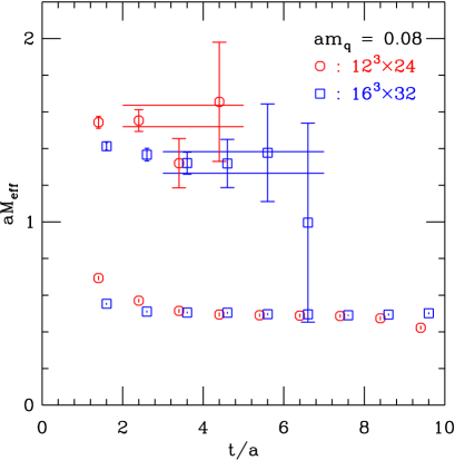
Figure 7: Ground- and excited-state effective masses for the pseudoscalars. Results for the $12^{3}\times 24$ (see Refs. BuGaGl04 ; BuGaGl04b ) and $16^{3}\times 32$ coarse lattices ($a\approx 0.15$ fm) are shown, along with horizontal lines displaying $M\pm\sigma_{M}$ from fits to the corresponding time intervals.

Figure 7 displays two pseudoscalar effective mass plots, one from one of the current data sets ($16^{3}\times 32$) and one from a previous set ($12^{3}\times 24$) at the same lattice spacing (see Refs. BuGaGl04 ; BuGaGl04b ). One can see that previously chosen fit ranges (for the $12^{3}$ lattices) may have been started at too small a value of $t$, apparently enhancing the resulting masses when compared to our current results. Since the physical spatial volume has been increased from 1.8 to 2.4 fm (the latter perhaps still being too small for excited-state spectroscopy; see Ref. SaSa05 ), one may be tempted to simply put this down as a finite-volume effect. However, since the later effective masses on the smaller lattices are consistent with the plateau found on the bigger ones, it is not easy to say whether this state is displaying effects due to the finite volume. The enhancement may also be due to higher state corrections, which still contribute since the minimum timeslice considered in the fit is too small. With better statistics on the $12^{3}$ lattices (to make up for the smaller number of spatial sites), we may end up finding a similar plateau to that seen on the $16^{3}$ lattices. Similar effects are seen for the vector mesons. We suspect that this poorer level of statistics for the $12^{3}$ lattices, and the subsequent choice of fit ranges, may account for most of the relative enhancement of our earlier results for the excited meson masses.

III.4 Chiral extrapolations of fine lattice results

Although we lack a third lattice spacing which would allow us to try to work in the continuum, we nevertheless attempt chiral extrapolations using the results from just our fine lattices (see Fig. 8). For the most part, we use simple linear extrapolations (interpolations for $\phi$) in $r_{0}^{2}M_{\pi}^{2}$ and, when doing so, avoid the low quark mass region ($r_{0}^{2}M_{\pi}^{2}<2.5$) for the pseudovectors since these suffer obviously large systematics there.

Assuming quenched chiral effects similar to those experienced by vector mesons BoChFa96 , we also allow for a $r_{0}M_{\pi}$ term (obviously negative) in the fits for the pseudovector extrapolations and include all points. We also try a quadratic fit in $r_{0}^{2}M_{\pi}^{2}$ for the scalars. These additional extrapolations are plotted as the bursts on the right of the column for each of these states. The right hand side of the plot shows the persistent difficulties of simulating pseudovector mesons in the quenched approximation. Dynamical simulations of these states appear not to suffer the same systematic enhancements MILC01 ; MILC04 . The extrapolations of the scalar appear more consistent with the $a_{0}(1450)$, a finding which appears consistent with unquenched results of simple $\bar{u}d$ scalars PrDaIz04 ; SuTsIs05 .

To the left in Fig. 8 we see that the results for the first-excited pseudoscalar and vector states agree with the experimental values (and dynamical calculations of excited pseudoscalars MILC04 ), while the ground-state vectors (except for the $\phi$) exhibit residual systematic effects, a common problem in the quenched approximation.

Given the fact that our results include (possibly large) systematic errors (quenching, finite volume, and chiral effects) which are not presently well understood, we point out that the correspondence between our masses and the physical ones in Fig. 8 should be viewed with some caution. Nevertheless, despite these possible pitfalls, it is remarkable that the mass splittings appear to be of the right size.

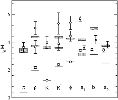
Figure 8: Chirally extrapolated (interpolated for $\phi$) results from our fine lattices ($20^{3}\times 32$, $a=0.119$ fm). Most extrapolations (circles, squares, and diamonds) are linear in $r_{0}^{2}M_{\pi}^{2}$. Those for the $a_{1}$, $b_{1}$, and $a_{0}$ are performed using only quark masses around the strange quark mass and heavier. The bursts on the right of the columns for these states are extrapolations including a $r_{0}M_{\pi}$ term (for $a_{1}$ and $b_{1}$) or a $r_{0}^{4}M_{\pi}^{4}$ term (for $a_{0}$), and all quark masses. The horizontal lines and shaded rectangles represent $M\pm\sigma_{M}$ experimental values.

IV Summary

We have presented ground- and excited-state meson masses from quenched lattice calculations using chirally improved quarks. Using a collection of linearly independent interpolating fields and the correlator matrix technique, we have been able to clearly separate the different mass eigenstates. Although it must be admitted that our statistical errors are still quite large, the masses we find for excited pseudoscalars are consistent with experimental values. The same is true for the excited vector mesons on our fine lattices. Results for the vectors on the coarser lattices suggest either that we have “missed” the first excitation (slightly lighter effective mass plateaus were seen in another eigenvalue, but without corresponding plateaus for the eigenvector) or that this state experiences significant discretization effects. The pseudovector and scalar mesons proved more difficult to handle. We could obtain few results for the excited states, virtually none below the strange quark mass. At low quark masses, already the ground states have problems, displaying significant quenching and/or finite-volume effects. Ultimately, these problems will only be overcome via simulations with better interpolators, larger physical volumes, and dynamical fermions.

- (1) G.P. Lepage, Nucl. Phys., Proc. Suppl. 106, 12 (2002).
- (2) M. Asakawa, T. Hatsuda, and Y. Nakahara, Prog. Part. Nucl. Phys. 46, 459 (2001).
- (3) C. Michael, Nucl. Phys. B259, 58 (1985).
- (4) M. Lüscher and U. Wolff, Nucl. Phys. B339, 222 (1990).
- (5) T. Burch et al. [Bern-Graz-Regensburg Collaboration], Phys. Rev. D 70, 054502 (2004).
- (6) T. Burch, C. Gattringer, L. Y. Glozman, C. Hagen, and C. B. Lang, Phys. Rev. D 73, 017502 (2006).
- (7) P. Weisz, private communication; see also K. J. Juge et al., arXiv:hep-lat/0601029.
- (8) S. Sasaki, T. Blum, and S. Ohta, Phys. Rev. D 65, 074503 (2002).
- (9) D. Brömmel et al. [Bern-Graz-Regensburg Collaboration], Phys. Rev. D 69, 094513 (2004); Nucl. Phys., Proc. Suppl. 129, 251 (2004).
- (10) T. Burch et al. [Bern-Graz-Regensburg Collaboration], Nucl. Phys., Proc. Suppl. 140, 284 (2005); Nucl. Phys. A755, 481 (2005).
- (11) C. R. Allton et al. [UKQCD Collaboration], Phys. Rev. D 47, 5128 (1993).
- (12) S. Basak et al. [Lattice Hadron Physics Collaboration (LHPC)], Phys. Rev. D 72, 094506 (2005); Phys. Rev. D 72, 074501 (2005); PoS LAT2005, 076 (2005).
- (13) S. Güsken, et al., Phys. Lett. B 227, 266 (1989).
- (14) C. Best et al., Phys. Rev. D 56, 2743 (1997).
- (15) M. Lüscher and P. Weisz, Commun. Math. Phys. 97, 59 (1985); Err.: 98, 433 (1985); G. Curci, P. Menotti, and G. Paffuti, Phys. Lett. B 130, 205 (1983); Err.: B 135, 516 (1984).
- (16) C. Gattringer, R. Hoffmann, and S. Schaefer, Phys. Rev. D 65, 094503 (2002).
- (17) C. Gattringer, Phys. Rev. D 63, 114501 (2001); C. Gattringer, I. Hip, and C.B. Lang, Nucl. Phys. B597, 451 (2001).
- (18) P.H. Ginsparg and K.G. Wilson, Phys. Rev. D 25, 2649 (1982).
- (19) C. Gattringer et al. [Bern-Graz-Regensburg Collaboration], Nucl. Phys. B677, 3 (2004); Nucl. Phys. B, Proc. Suppl. 119, 122 (2003); Nucl. Phys. B, Proc. Suppl. 119, 796 (2003).
- (20) C. Gattringer, P. Huber, and C.B. Lang, Phys. Rev. D 72, 094510 (2005).
- (21) T. Burch, C. Hagen, D. Hierl, A. Schäfer, C. Gattringer, L. Y. Glozman, and C. B. Lang, Proc. Sci. LAT2005, 097 (2005).
- (22) M. Booth, G. Chiladze, and A. F. Falk, Phys. Rev. D 55, 3092 (1997).
- (23) S. Prelovsek, C. Dawson, T. Izubuchi, K. Orginos, and A. Soni, Phys. Rev. D 70, 094503 (2004); S. Prelovsek, Proc. Sci. LAT2005, 085 (2005).
- (24) H. Suganuma, K. Tsumura, N. Ishii, and F. Okiharu, Proc. Sci. LAT2005, 070 (2005).
- (25) K. Sasaki and S. Sasaki, Phys. Rev. D 72, 034502 (2005); Proc. Sci. LAT2005, 060 (2005).
- (26) C. W. Bernard et al., Phys. Rev. D 64, 054506 (2001).
- (27) C. Aubin et al., Phys. Rev. D 70, 094505 (2004);