Simulating the scalar field on the fuzzy sphere

Abstract:

The properties of the $\phi^{4}$ scalar field theory on a fuzzy sphere are studied numerically. The fuzzy sphere is a discretization of the sphere through matrices in which the symmetries of the space are preserved. This model presents three different phases: uniform and disordered phases, as in the usual commutative scalar field theory, and a non-uniform ordered phase related to UV-IR mixing like non-commutative effects. We have determined the coexistence lines between phases, their triple point and their scaling.

PoS(LAT2005)262

1 Introduction

The fuzzy approximation scheme [1] consists in approximating the algebra of functions on a manifold with a finite dimensional matrix algebra instead of discretising the underlying space as a lattice approximation does.

Here we report our results for a hermitian scalar field on the fuzzy sphere. We find the collapsed phase diagram and in particular we calculate the uniform ordered/non-uniform ordered line that was absent in [2].

The current study could be relatively easily repeated for a hermitian scalar field on other fuzzy spaces. The simplest extension would be to fuzzy $\mbox{\openface CP}^{\rm N}$. Some variants of the scheme can be applied to fuzzy versions of $S^{3}$ and $S^{4}$[3]. The study reveals that the non-uniform disordered phase lines should correspond to a pure matrix model transition.

As an approximation scheme, this “fuzzification” is well suited to numerical simulations of field theories [4]. As a test run, the first fuzzy approximation to be investigated should be the simplest one, that of the two dimensional sphere $\mbox{\openface CP}^{1}=S^{2}$. Both the two–dimensional commutative and Moyal planes can be viewed as the limits of a fuzzy sphere of infinite radius.

2 The two dimensional $\phi^{4}$ Model and its fuzzy version

We are interested in the model:

$$S[\Phi]=Tr\left[a\,\Phi^{\dagger}\left[L_{i},\left[L_{i},\Phi\right]\right]+b\Phi^{2}+c\Phi^{4}\right],$$ (1)

where $\Phi$ is a Hermitian matrix of size $N$, $b$ and $c$ are mass and coupling parameters respectively. $L_{i}$ is the angular momentum generator in the $N$ dimensional unitary irreducible representation of $SU(2)$. Since a rescaling of $\Phi$ will allow us to set $a=1$, the entire phase diagram can be explored by ranging through all real values of $b$ and positive values of $c$. The conventions of [2] are $a=\frac{4\pi}{N}$, $b=arR^{2}$, $c=a\lambda R^{2}$.

The infinite matrix limit of the action can be taken and corresponds to a real scalar field $\phi$ on a round sphere of radius $R$ and Euclidean action

$$S[\phi]=\int_{S^{2}}d^{2}{\bf n}\left(\phi{\cal L}^{2}\phi+rR^{2}\phi^{2}+\lambda R^{2}\phi^{4}\right)$$ (2)

where ${\cal L}^{2}=\sum_{i=1,3}{\cal L}_{i}^{2}$ and ${\cal L}_{i}$ are the usual angular momentum generators.

The eigenvectors of $\left[L_{i},\left[L_{i},\cdot\right]\right]$ in (1) are the polarization tensors $\hat{Y}_{lm}$ (normalised so that $\frac{4\pi}{N}\mathrm{Tr}(\hat{Y}_{lm}^{\dagger}\hat{Y}_{lm})=1$) and it has eigenvalues $l(l+1)$ with degeneracy $2l+1$. This is precisely the spectrum of the Laplacian $\mathcal{L}^{2}$ on the commutative sphere truncated at angular momentum $N-1$.

This particular model was chosen because of its simplicity. The diagrammatic expansion of the model (2) has only one divergent diagram, the tadpole diagram, is Borel resumable, and defines the field theory entirely. In the fuzzy version, the tadpole splits into planar and non-planar tadpoles, which are also the only diagrams that diverge in the infinite $N$ limit. Their difference is finite and nonlocal and is responsible for the UV/IR mixing phenomena of the disordered phase [6].

Even though the scalar field on either commutative or fuzzy spheres cannot have a phase transition, since they have finite volume or a finite number of degrees of freedom, phase transitions may be found when the matrix dimension or the radius of the sphere become infinite.

The fuzzy sphere can be recognized by introducing coordinates $\left(X_{1},X_{2},X_{3}\right)$ proportional to the angular momentum operators

$$X_{i}=\frac{2R}{\sqrt{N^{2}-1}}L_{i}.$$

They must satisfy the algebra

$$\ X^{2}_{1}+X^{2}_{2}+X^{2}_{3}=R^{2}{\bf 1},\hskip 28.45274pt\left[X_{i},X_{j}\right]=i\frac{\Theta}{R}\epsilon_{ijk}X_{k}$$

where $\Theta=\frac{2R^{2}}{\sqrt{N^{2}-1}}$ is the parameter of non-commutativity, $R$ is the radius of the sphere and ${\bf 1}$ is the unit operator. The non-commutativity parameter depends on the matrix size, $N$, and the radius of the sphere, $R$. By taking different limits we can access different spaces:

$N$	$R$	$\Theta$	Limit
$N$	constant = $R$	$2R^{2}/\sqrt{N^{2}-1}$	Fuzzy Sphere
$\infty$	constant = $R$	$0$	Commutative Sphere
$\infty$	$\infty$	$0$	Commutative plane
$\infty$	$\infty$	constant = $\theta$	Moyal Plane

2.1 Order parameters

A suitable set of order parameters can be identified from the coefficients of a mode decomposition in terms of the polarization tensors basis [5]

$$\Phi=Tr(\Phi)\frac{\bf 1}{N}+\frac{12}{N(N^{2}-1)}\rho_{a}L_{a}+\sum_{l=2}^{N-1}\sum_{m=-l}^{+l}c_{lm}\hat{Y}_{lm}.$$ (3)

We have separated explicitly $l=0$ and $l=1$ from the expansion to identify two observables whose expectation values we used to identify the respective phases. The observables are $|Tr(\Phi)|$ and $\rho^{2}:=\rho_{a}\rho_{a}=\displaystyle\sum_{a=1}^{3}(Tr(L_{a}\Phi))^{2}$. The total power in all coefficients is given by $Tr(\Phi^{2})=\frac{1}{N}(Tr(\Phi))^{2}+\frac{12}{N(N^{2}-1)}\rho^{2}+\frac{N}{4\pi}\displaystyle\sum_{l=2}^{N-1}\displaystyle\sum_{m=-l}^{l}|c_{lm}|^{2}$ and can be used to estimate the importance of the neglected higher modes.

2.2 The phases

This model (1) presents three phases. As a generic illustration of their properties, Fig. 1(a) and Fig.1(b) show the dependence on the mass parameter $b$ of the probability distributions of $Tr(\Phi)$ and $\rho$, respectively, for $\left\{a=1,\ c=40,\ N=4\right\}$.

Disordered: Found for $|b|$ “small”, the configurations fluctuate close to $\Phi=0$. This is confirmed on the figure, $<|Tr(\Phi)|>\sim<\rho>\sim 0$, but also $<Tr(\Phi^{2})>\sim 0$ (not shown).

Non-uniform ordered: As $|b|$ increases, the figure shows multiple symmetric peaks for the probability distribution of $Tr(\Phi)$ whose height decreases with increasing $|Tr(\Phi)|$, and multiple peaks not centered near zero for $\rho$. Furthermore $Tr(\Phi^{2})$ is much larger than both $\frac{<|Tr(\Phi)|>^{2}}{N}$ and $<\rho>$ so that higher modes actually dominate. In particular, the most probable configuration is not rotationally invariant and we have spontaneous breakdown of rotational invariance. The probability distribution of $Tr(\Phi)$ has $N+1$ symmetric peaks located approximately at $(N-2k)\sqrt{-b/2c}$ where $k=0,1,\dots,N$, while the probability distributions of $\rho$ and $S[\Phi]$ have $(N+1)/2$ peaks for $N$ odd and $N/2+1$ for $N$ even.

Uniform ordered: As $|b|$ becomes large, the figure shows two symmetric peaks for the probability distribution of $Tr(\Phi)$ corresponding to the outer peaks of the non-uniform ordered phase and located approximately at $Tr(\Phi)\sim\pm N\sqrt{-b/2c}$, but just one peak near zero for $\rho$. Furthermore, $<Tr(\Phi^{2})>\sim<Tr(\Phi)>^{2}/N$ indicating that the power in higher modes is negligible. This is generic and indicates that $\Phi\sim\sqrt{-b/2c}\,{\bf 1}$ and the rotational symmetry is thus restored.

 

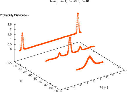
(a) Probability distribution of $Tr(\Phi)$

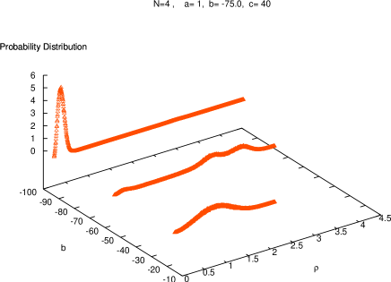
(b) Probability distribution of $\rho$.

Figure 1: Figures (a) and (b) show the typical behavior of the observables $Tr(\Phi)$ and $\rho$ in a region of the phase diagram where decreasing $b$ passes the system through the three phases.

3 Simulation and Results: The specific heat and the phase diagram

We are interested in the phase diagram of the model (1). To identify it, we used the coordinates in parameter space of the peaks of the specific heat, $C:=<S^{2}>-<S>^{2}$. The relevant set of parameters is $\left\{N,b,c\right\}$ where $b$ and $c$ depend implicitly in $R$. It is possible to further reduce by one the number of parameters by finding a scaling $\left\{b,c\right\}\to\left\{bN^{\theta_{b}},cN^{\theta_{c}}\right\}$. If we find such $\theta_{b}$ and $\theta_{c}$, the model becomes independent of $N$ and automatically yields an infinite matrix limit.

The simulations show that in the non–uniform ordered phase, the fuzzy kinetic term (proportional to $a$ in (1)), is negligible compared to the potential term (the other terms). There exists an exact solution for the corresponding limit of $a=0$ in the large $N$ limit called the pure potential model [7]. This model predicts a third order phase transition between a disordered and non–uniform ordered phase at $c=b^{2}/4N$. Figure 2 confirms numerically the convergence of the disordered/non–uniform ordered transition towards this exact critical line of the pure potential model.

Figure 2: Plot of the specific heat at the disordered/non–uniform ordered transition for increasing $N$ and its $N\to\infty$ limit, the exact pure potential model.

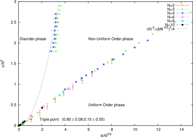
Figure 3: Phase diagram obtained from Monte–Carlo simulations of the model (1)

Numerically, it is not difficult to find the coexistence curve between the uniform ordered and disordered phases which exist for low values of $c$. On the other hand, the coexistence curve between the two ordered phases is difficult to evaluate because it involves a jump in the field configuration and tunnelling over a wide potential barrier.

The phase diagram obtained by Monte Carlo simulations with the Metropolis algorithm is shown on figure 3. That plot shows the phase diagram for the model (1). The data have been collapsed using the scaling form defined above with $\theta_{b}=-3/2$ and $\theta_{c}=-2$. It is remarkable that this scaling also works for the exact solution of the pure model potential.

4 Conclusions

The numerical study showed three different phases. In one of those phases, which does not exist in the commutative planar $\lambda\phi^{4}$ theory, the rotational symmetry is spontaneously broken. The other two phases have qualitatively the same character as the phases of this latter model. The three coexistence curves intersect at a triple point given by

$$(b_{{}_{T}},c_{{}_{T}})=(-0.15N^{3/2},0.8N^{2}).$$ (4)

Those three curves and the triple point collapse using the same scaling function of $N$ and thus give a consistent $N\to\infty$ limit. Thus, all three phases, and in particular the new uniform disordered phase, and the triple point survive in the limit. We will discuss these issues more completely in Ref. [8].

Acknowledgements

We wish to thank W. Bietenholz and J. Medina for helpful discussions.

References

- [1] J. Hoppe, MIT Ph.D. thesis (1982); J. Hoppe, Elem. Part. Res. J. (Koyoto) 80 145 (1989). H. Grosse and P. Presnajder, Lett.Math.Phys. 33, 171 (1995); H. Grosse, C. Klimčík and P. Presnajder, Commun.Math.Phys. 178,507 (1996); 185, 155 (1997); H. Grosse and P. Presnajder, Lett.Math.Phys. 46, 61 (1998) and ESI preprint, (1999); H. Grosse, C. Klimcík, and P. Presnajder, hep-th/9602115 and Commun.Math.Phys. 180, 429 (1996); H. Grosse, C. Klimcík, and P. Presnajder, in Les Houches Summer School on Theoretical Physics, 1995, hep-th/9603071. S. Baez, A. P. Balachandran, S. Vaidya and B. Ydri Commun.Math.Phys. 208, 787-798 (2000); . P. Balachandran, T.R.Govindarajan and B. Ydri, Mod.Phys.Lett. A15 1279 (2000); G.Alexanian, A.P.Balachandran, G.Immirzi and B.Ydri J.Geom.Phys. 42 28–53 (2002); Badis Ydri hep-th/0110006.
- [2] X. Martin, A matrix phase for the scalar field on the fuzzy sphere.JHEP 0404 (2004) 077 [hep-th/0402230].
- [3] B. P. Dolan and D. O’Connor, JHEP 0310, 060 (2003). J. Medina and D. O’Connor, JHEP 0311, 051 (2003).
- [4] T. Azuma, S. Bal, K. Nagao and J. Nishimura hep-th/0401038.
- [5] D.A. Varshalovich, A.N. Moskalev, V.K. Khersonskii, Quantum Theory of Angular Momentum, World Scientific Pub Co Inc. October (1988).
- [6] Chong-Sun Chu, John Madore, Harold Steinacker Scaling Limits of the Fuzzy Sphere at one Loop JHEP 0108 038 (2001) [hep-th/0106205]; B.P. Dolan, D. O’Connor and P. Prešnajder, Matrix models on the fuzzy sphere and their continuum limits, JHEP 03 013 (2002) [hep-th/0109084].
- [7] E.Brézin, C. Itzykson, G. Parisi and J. B. Zuber, Planar diagrams. Comm. Math. Phys. 59, 35 (1978). P. Di Francesco, P. Ginsparg, J. Zinn-Justin, 2D Gravity and Random Matrices. hep-th/9306153. Pavel Bleher, Alexander Its, Double scaling limit in the random matrix model: the Riemann-Hilbert approach. [math-ph/0201003].
- [8] Fernando García Flores, Xavier Martin and Denjoe O’Connor in preparation.