DIRAC EIGENMODES IN AN ENVIRONMENT OF DYNAMICAL FERMIONS

We discuss some properties of zero and near-zero modes of the Dirac operator, as observed in a recent simulation of 2-flavor QCD. The quarks have been implemented with the so-called Chirally Improved Dirac operator, which obeys the Ginsparg-Wilson relation to a good approximation. We present geometrical and statistical properties of these eigenmodes and eigenvalues.

1 Motivation and introduction

Throughout the last decades of lattice QCD topological excitations have played a crucial and sometimes controversial role. It is natural, in particular in view of the purpose of this volume in honor of Adriano Di Giacomo, that they are a topic also here.$\!{}^{{\bf?}}$

The topological charge of a gauge configuration is a well-defined concept only in the continuum and for differentiable fields. In quantum field theory the gauge configurations are in general non-differentiable. Lattice discretization turns out to be an ideal tool for doing a non-perturbative gauge invariant regularization of QCD; however introducing a smallest distance thus we lose the continuum in such studies. In fact, a constructive definition of the topological charge is only possible when certain smoothness requirements are introduced.$\!{}^{{\bf?}}$ It is also quite demanding to implement in actual calculations.

For that reason various other methods have been addressed, among them ultra-local definitions of the topological charge density $\!{}^{{\bf?}}$, together with various modifications.$\!{}^{{\bf?}}$ When considering the total topological charge of gauge field configurations cooling techniques have been employed in the attempt to smoothen the gauge configuration and get rid of discretization artefacts like dislocations for example.

One of the cleanest tools for identifying the topological charge is through the measurement of a costly fermionic observable: eigenmodes of the Dirac operator. The Atiyah-Singer index theorem $\!{}^{{\bf?}}$ relates the topological charge of a gauge configuration with the difference between the number of left-handed and right-handed zero modes. Unfortunately the discretization in itself complicates this approach. In the continuum zero modes also have definite chirality. Dirac operators on the lattice violate explicitly chiral symmetry, as it is defined in the continuum. Only recently one has rediscovered a relation $\!{}^{{\bf?}}$ generalizing the continuum chiral symmetry to the lattice by adding a local piece, that vanishes in the continuum. In its simplest form this so-called Ginsparg-Wilson (GW) relation reads

$$\{D,\,D^{\dagger}\}=D\,D^{\dagger}\;,$$ (1)

and it may be associated with a symmetry transformation $\!{}^{{\bf?}}$, that becomes the chiral transformation in the continuum limit. This symmetry protects the zero modes, which now have definite chirality even on the lattice.

Dirac operators obeying the GW relation may thus be utilized to identify the topological charge of a gauge configuration by identifying the number and chirality of the zero modes. Various GW type Dirac operators have been introduced: Domain Wall Fermions $\!{}^{{\bf?},{\bf?},{\bf?},{\bf?}}$, the Perfect Fermions $\!{}^{{\bf?},{\bf?}}$ or the Chirally Improved (CI) Fermions.$\!{}^{{\bf?},{\bf?}}$ They all fulfill the GW condition not exactly but in some approximation. They are also more complicated to deal with than the simple Wilson operator, having many more coupling terms or introducing an extra dimension. The only known explicit and exact realization, the so-called overlap operator $\!{}^{{\bf?},{\bf?}}$, is even more expensive to implement in computer simulations.

With better chiral behavior there comes an associated extra advantage. The simple Wilson Dirac operator has scattered real modes near the origin in the complex plane. These become true zero modes in the continuum limit. At present day lattice spacing values they lead to spurious zeros even at non-zero mass of the quark fields (see, however, Ref. $\!{}^{{\bf?}}$). Improving the chirality also improves this situation. GW type fermions have the chance to allow for a better approach to the chiral limit, i.e., to come closer to the physical value of the pion mass without having to go to very large and fine lattices. Exact GW fermions have no spurious modes, i.e., no eigenvalues below the values of the mass parameter.

Real zero modes may thus be used to obtain the total topological change; its fluctuation gives the topological susceptibility which, in the quenched case is related to the mass of the $\eta^{\prime}$ (cf. Refs. $\!{}^{{\bf?},{\bf?}}$). For the dynamical case its dependence on $N_{f}$ and $m$ has been discussed recently.$\!{}^{{\bf?},{\bf?},{\bf?},{\bf?}}$

So-called near zero modes are associated with complex conjugate pairs of small eigenvalues. Spontaneous chiral symmetry breaking relates their density to the value of the chiral condensate via the Banks-Casher relation.$\!{}^{{\bf?}}$ Random matrix theory (RMT) describes the probability density of such eigenvalues for operators belonging to various universality classes including that of the QCD Dirac operator. Such a probability density depends on the topological sector, the quark mass and the volume.$\!{}^{{\bf?},{\bf?}}$

For all these reasons zero modes are of high interest: both, leading to important physical observables, and as a technical tool to identify the behavior and quality of the simulation.

Table 1: Parameters for the simulations; the first column denotes the run, for later reference. The gauge coupling is $\beta_{1}$, the bare quark mass parameter $am$, HMC-time denotes the length of the run (number of trajectories), and the lattice spacing has been determined via the Sommer parameter.

#	$L^{3}\times T$	$\beta_{1}$	$a\,m$	HMC-time	$a_{S}$[fm]
a	$12^{3}\times 24$	5.2	0.02	463	0.115(6)
b	$12^{3}\times 24$	5.2	0.03	363	0.125(6)
c	$12^{3}\times 24$	5.3	0.04	438	0.120(4)
d	$12^{3}\times 24$	5.3	0.05	302	0.129(1)
e	$8^{3}\times 16$	5.3	0.05	1245	0.135(3)

2 Dynamical fermion simulation

The CI Dirac operator $D_{\textrm{\scriptsize{CI}}}$ was constructed by writing a general ansatz for the Dirac operator

$$D_{ij}=\sum_{k=1}^{16}\alpha^{k}_{ij}(U)\,\Gamma_{k}\;,$$ (2)

where $\Gamma_{k}$ $(k=1\ldots 16)$ are the 16 elements of the Clifford algebra and $\alpha^{k}_{ij}(U)$ are linear combinations of path ordered products of links $U$ connecting lattice site $i$ with site $j$. Inserting $D$ into the GW relation and solving the resulting algebraic equations for the coefficients of the linear combinations yields $D_{\textrm{\scriptsize{CI}}}$. In principle this can be an exact solution, but that would require an infinite number of terms. In practice the number of terms is finite and the operator is a truncated series solution to the GW relation.$\!{}^{{\bf?},{\bf?}}$

CI fermions have been already extensively tested in quenched calculations (see, e.g., Ref. $\!{}^{{\bf?}}$). In these tests it was found that one can go to quark masses below 300 MeV without running into the problem of exceptional configurations (spurious zero modes). On quenched configurations pion masses down to 280 MeV could be reached on lattices of size $16^{3}\times 32$ (lattice spacing 0.148 fm) and about 340 MeV on $12^{3}\times 24$ lattices.

In recent work $\!{}^{{\bf?},{\bf?}}$ we have studied the CI fermions in a dynamical simulation of QCD with two light flavors. All technicalities are discussed in Ref. $\!{}^{{\bf?}}$. For definiteness we just mention that our gauge action is the Lüscher-Weisz action $\!{}^{{\bf?}}$, that we used stout smearing $\!{}^{{\bf?}}$ of the gauge fields as part of the Dirac operator definition, and that the Hybrid Monte Carlo method was implemented to deal with the dynamics of the fermions. The lattices were (up to now) of moderate size: $8^{3}\times 16$ and $12^{3}\times 24$, for lattice spacings between 0.11 and 0.14 fm. Table 1 summarizes the simulation parameters of the runs discussed here (see, however, Ref. $\!{}^{{\bf?}}$ for a more complete list).

3 Zero modes and near zero modes

3.1 Isosurface plots

When dealing with zero modes some visualization of the geometric structure may be desirable. The instantons, which provide finite energy analytic solutions to the Yang-Mills field equations, are prime candidates for the topological excitations. In some scenarios a gas of instantons $\!{}^{{\bf?}}$ supposedly leads to chiral symmetry breaking. In this picture the low-lying near-zero modes come from overlapping instanton – anti-instanton pairs.

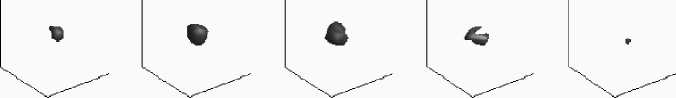
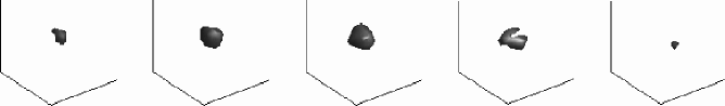
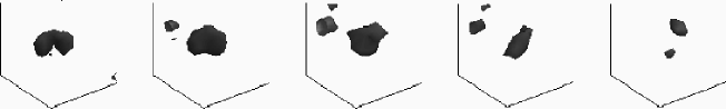
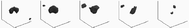
Figure 1: Iso-surfaces at time slices close to the maximum of the scalar density. Rows 1 and 2: typical case of a single lump; row 1: $\rho_{0}$ ($I=15.6$), row 2: $\rho_{5}$ ($I=12.1$). Rows 3 and 4: several lumps in one eigenvector; row 3: $\rho_{0}$ ($I=3.2)$, row 4: $\rho_{5}$ ($I=2.4$).

A possible analysis tool is to introduce the gauge invariant density of the corresponding eigenvectors $\psi_{c\alpha}(x)$, in particular

$$\rho_{0}(x)\equiv\sum_{c,\alpha}{\overline{\psi}}_{c\alpha}(x)\psi_{c\alpha}(x)\;,\;\;\rho_{5}(x)\equiv\sum_{c,\alpha,\beta}{\overline{\psi}}_{c\alpha}(x)(\gamma_{5})_{\alpha\beta}\psi_{c\beta}(x)\;,$$ (3)

with the normalization $\sum_{x}\rho_{0}(x)=1$ ($c$ denotes the color index and $\alpha,\beta$ the Dirac indices). The sum $\sum_{x}\rho_{5}(x)$ gives the chirality $\langle\psi|\gamma_{5}|\psi\rangle$ of the mode. For exactly zero modes of an exact GW operator one has $\rho_{0}(x)=\pm\rho_{5}(x)$ locally.

For approximate GW operators like ours, the real eigenvalues of $D$ are not exactly zero, but the corresponding eigenmodes are the only ones with non-vanishing chirality. As a typical example let us study two eigenvectors corresponding to slightly different but real eigenvalues of one configuration. In Fig. 1 we compare iso-surfaces at $\rho_{0}=0.25$ of the maxima values, shown as 3-cuts at time slices close to the density maxima. Comparing the density values for $\rho_{0}$ with $\rho_{5}$ we find that the chirality of the mode is indeed located mainly where the scalar density is concentrated. The two sets of plots also show typical distributions: the zero modes are as often located in individual blobs as they are distributed on several such lumps. Note, that we discuss here eigenvectors for individual real (“zero”) modes and not sums of such.

The inverse participation ratio

$$I_{k}=V\,\sum_{x}\rho_{k}(x)^{2}$$ (4)

($V$ is the lattice volume in units of the lattice spacing) gives a global information on the localization of the eigenmode. Its value ranges between $V$ denoting point localization and $1$ for an uniformly spread mode. If a mode is uniformly distributed on $N$ sites it has $I=V/N$, thus $1/I$ indicates the fraction of the volume occupied by the mode. Fig. 2 shows the histogram for the inverse participation ratio measured on the zero mode eigenvectors for the run (a). The values of $I_{0}$ for the zero modes are quite similar to the results for quenched simulations for comparable lattice size and spacing.$\!{}^{{\bf?}}$ The average values for run (a) are $I_{0}=14.0(3.4)$ and $I_{5}=8.7(2.0)$.

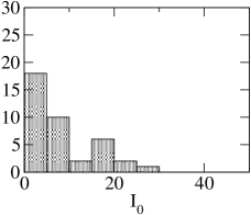
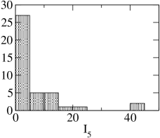
Figure 2: Histogram for the inverse participation ratios $I_{0}$ and $I_{5}$for the zero modes in run sequence (a).

In Ref. $\!{}^{{\bf?}}$ it was observed that the lumps may change their positions when the boundary conditions change. A possible interpretation is that the lumps carry fractional topological charges. We normally use anti-periodic boundary conditions in time direction. However for a subset of 10 of our configurations we also determined the eigensystem for periodic b.c.; in one of those we observed a change in the number of zero modes. For the other configurations the number stayed the same and the density showed only very little change.

Tunneling between different topological sectors appears to be a problem for HMC implementations of the overlap action; various intricate methods have been suggested to deal with it. We do not seem to have such a problem and observe frequent tunneling. We determined the eigenvalues and thus the topological charge only for every 5th configuration. Comparing the number of changes of the topological sector we get (for the runs (a,b,d) and (e)) between 12 and 19 such changes along a HMC-time distance of 100, without obvious correlation to the run parameters. These values are a lower bound for the actual number of tunneling events. As is well-known from experience with other Dirac operators, when evaluated over longer HMC-periods than the ones available to us, the tunneling frequency may show much longer correlation time.$\!{}^{{\bf?},{\bf?}}$ One may expect then longer wavelength fluctuations in the topological charge than observed here.$\!{}^{{\bf?}}$

3.2 Density of near zero modes

Random matrix theory gives the density distributions of the low-lying non-zero eigenvalues in universality classes depending on the general symmetry properties of the Dirac operator. The densities should scale with a scaling variable proportional to $V\,\mathrm{Im}(\lambda)$. The proportionality constant may be related to the fermion mass and the chiral condensate.$\!{}^{{\bf?},{\bf?}}$ Although we have limited statistics, in particular for the larger lattice, we still identify such volume scaling as can be seen in Fig. 3.

In order to exhibit the scaling behavior we plot the abscissa scaled according to the respective volume. We also indicate the positions of the mean values of the histograms and find good agreement with the expected volume scaling within the limited statistics.

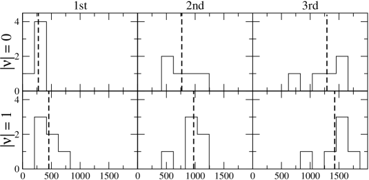
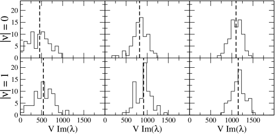
Figure 3: Density of the $\mathrm{Im}(\lambda)$ values of the 1st, 2nd and 3rd lowest non-zero modes for the runs (d) and (e) at $\beta_{1}=5.3$ and $am=0.05$ for two volumes (top: $V_{12}=12^{3}\times 24$, bottom: $V_{8}=8^{3}\times 16$) in the sectors of topological charge $\nu=0$ and $\nu=1$. The abscissa of histograms are scaled with the volume.

3.3 More on the smallest eigenmodes

Recently the distribution of the smallest eigenvalue of the hermitian Wilson Dirac operator has been studied in a dynamical fermion simulation $\!{}^{{\bf?}}$ for large lattices and the standard Wilson Dirac operator. There it was found that the median of that distribution is near the value of the so-called AWI-mass, the physical quark mass determined from the PCAC-relation. The width of the distribution appears to scale proportional to $a/\sqrt{V}$ (in physical units). This width gives information on the range of mass values accessible in such simulations. The eigenvalues occurring to the left of the AWI-mass lead to the so-called spurious zero modes, i.e., a zero of the Dirac operator at positive quark masses and thus a spurious singularity in the quark propagator.

Let us briefly consider the situation for a perfect GW operator, in particular one following the simple form Eq. 1, for zero mass. The eigenvalue in that case lie on a circle with radius 1 and center at 1 in the complex plane. One may add a mass through

$$D_{GW}(m)=\left(1-\frac{m}{2}\right)D_{GW}+m\mathbf{1}\;.$$ (5)

The smallest (in terms of distance from the origin) eigenvalue of $D_{GW}(m)$ is either real $\lambda_{\textrm{\scriptsize{min}}}=m$ or on the circle at, say $\lambda_{\textrm{\scriptsize{min}}}=m\pm\mathrm{i}\epsilon$. The probability distribution of the density of $|\lambda_{\textrm{\scriptsize{min}}}|$ at finite volume consists of a delta-function at $|\lambda_{\textrm{\scriptsize{min}}}|=m$ (from the exact zero modes) and the folded distribution of the lowest non-zero mode, known from RMT.$\!{}^{{\bf?},{\bf?}}$

Figure 4: Sketch of the distribution of the smallest eigenvalue $|\lambda|$ for a GW Dirac operator $D_{\textrm{\scriptsize{GW}}}(m)$ on a finite lattice. The vertical thick line at $\lambda=m$ symbolizes the delta function due to the real (“zero”) modes. The shaded area represents the modes on the circle, which dominate in the infinite volume limit; in this limit, the width of this part of the distribution shrinks to zero $\propto 1/V$.

Fig. 3.3 gives a sketch of the situation for an exact GW operator. The weight of the delta-function is proportional to the number of configurations with at least one exact zero mode and thus related to the finite volume topological susceptibility. Assuming the topological charge $|\nu|$ has Gaussian distribution with $\langle\nu^{2}\rangle=\chi V$ the probability of the $\nu=0$ sector is $P=1/\sqrt{2\pi\langle\nu^{2}\rangle}\propto 1/\sqrt{V}$; this defines the normalization of the nearest non-zero modes distribution. (Note, however, that the susceptibility for dynamical fermions vanishes with the fermion mass $\!{}^{{\bf?},{\bf?},{\bf?},{\bf?},{\bf?}}$.) The weight of the delta-function is $1-P$.

In Fig. 5 we show the distribution obtained for two of our simulation runs. Only the eigenvalues below the value of the AWI-mass are spurious modes. The situation is similar to that of an exact GW operator. In the study for dynamical Wilson fermions the median of the corresponding distribution was close to the value of the AWI mass. In our case, the AWI-mass is much below that median. This motivates the use of GW type Dirac operators.

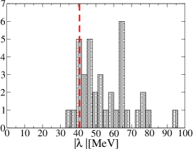
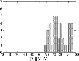
Figure 5: Distribution of the absolute value of the smallest eigenmodes for run (a) (l.h.s.) and (b) (r.h.s). The vertical, dotted lines indicate the values of the AWI-mass as determined in Ref. ²⁹. The quark mass has been converted to physical units using the lattice spacing determined from the Sommer parameter.

4 Summary

We have implemented the Chirally Improved Dirac operator, obeying the GW condition to a good approximation, in a simulation with two species of mass-degenerate light quarks. Studying the low-lying eigenmodes allows us to check the quality of the Dirac operator and the simulation. Here we surveyed some details concerning the geometrical properties of these eigenmodes and the probability distribution.

References

References

- [1] M. Creutz, Fun with Dirac eigenvalues, 2005 [arXiv:hep-lat/0511052].
- [2] M. Lüscher, Commun. Math. Phys. 85, 39 (1982).
- [3] P. Di Vecchia et al., Nucl. Phys. B192, 392 (1981).
- [4] T. DeGrand, A. Hasenfratz, and T. G. Kovacs, Nucl. Phys. B505, 417 (1997).
- [5] M. Atiyah and I. M. Singer, Ann. Math. 93, 139 (1971).
- [6] P. H. Ginsparg and K. G. Wilson, Phys. Rev. D 25, 2649 (1982).
- [7] M. Lüscher, Phys. Lett. B 428, 342 (1998).
- [8] D. B. Kaplan, Phys. Lett. B 288, 342 (1992).
- [9] V. Furman and Y. Shamir, Nucl. Phys. B439, 54 (1995).
- [10] Y. Aoki et al., Lattice QCD with two dynamical flavors of domain wall quarks, 2004 [arXiv:hep-lat/0411006].
- [11] D. J. Antonio et al., Proc. Sci. LAT2005, 080 (2005).
- [12] P. Hasenfratz and F. Niedermayer, Nucl. Phys. B 414, 785 (1994).
- [13] A. Hasenfratz, P. Hasenfratz, and F. Niedermayer, Simulating full QCD with the fixed point action, 2005 [arXiv:hep-lat/0506024].
- [14] C. Gattringer, Phys. Rev. D 63, 114501 (2001).
- [15] C. Gattringer, I. Hip, and C. B. Lang, Nucl. Phys. B597, 451 (2001).
- [16] R. Narayanan and H. Neuberger, Phys. Lett. B 302, 62 (1993); Nucl. Phys. B443, 305 (1995).
- [17] H. Neuberger, Phys. Lett. B 417, 141 (1998); Phys. Lett. B 427, 353 (1998).
- [18] L. D. Debbio et al., Stability of lattice QCD simulations and the thermodynamic limit, 2005 [arXiv:hep-lat/0512021].
- [19] E. Witten, Nucl. Phys. B156, 269 (1979).
- [20] G. Veneziano, Nucl. Phys. B159, 213 (1979); Phys. Lett. B 95, 90 (1980).
- [21] L. Giusti et al., Nucl. Phys. B628, 234 (2002).
- [22] E. Seiler, Phys. Lett. B 525, 355 (2002).
- [23] L. Giusti, G. Rossi, and M. Testa, Phys. Lett. B 587, 157 (2004).
- [24] M. Lüscher, Phys.Lett. B 593, 296 (2004).
- [25] T. Banks and A. Casher, Nucl. Phys. B 169, 103 (1980).
- [26] S. M. Nishigaki, P. H. Damgaard, and T. Wettig, Phys. Rev. D 58, 087704 (1998).
- [27] P. H. Damgaard and S. M. Nishigaki, Phys. Rev. D 63, 045012 (2001).
- [28] C. Gattringer et al., Nucl. Phys. B677, 3 (2004).
- [29] C. B. Lang, P. Majumdar, and W. Ortner, Proc. Sci. LAT2005, 124 (2005); Proc. Sci. LAT2005, 131 (2005).
- [30] C. B. Lang, P. Majumdar, and W. Ortner, QCD with two dynamical flavors of chirally improved quarks, 2005 [arXiv:hep-lat/0512014].
- [31] M. Lüscher and P. Weisz, Commun. Math. Phys. 97, 59 (1985).
- [32] C. Morningstar and M. Peardon, Phys.Rev. D 69, 054501 (2004).
- [33] T. Schäfer and E. V. Shuryak, Rev. Mod. Phys. 70, 323 (1998).
- [34] C. Gattringer et al., Nucl. Phys. B (Proc. Suppl.) 106, 551 (2002); Nucl. Phys. 617, 101 (2001); Nucl. Phys. 618, 205 (2001).
- [35] C. Gattringer, Phys. Rev. D 67, 034507 (2003). C. Gattringer and R. Pullirsch, Phys. Rev. D 69, 094510 (2004).
- [36] B. Alles et al., Phys.Rev. D 58, 071503 (1998).
- [37] R. J. Crewther, Phys. Lett. B 70, 349 (1977).
- [38] H. Leutwyler and A. Smilga, Phys. Rev. D 46, 5607 (1992).
- [39] C. Gattringer, R. Hoffmann, and S. Schaefer, Phys. Lett. B 535, 358 (2002).
- [40] L. D. Debbio and C. Pica, JHEP 02, 003 (2004).
- [41] L. D. Debbio, L. Giusti, and C. Pica, Phys.Rev.Lett. 94, 032003 (2005).