Ever since the pioneering work by Creutz [1] the approach to asymptotic scaling, and thus the continuum limit, was one of the central issues in studies of gauge theories on the lattice. Although the first results were promising, the lack of asymptotic scaling of physical observables has been observed in SU(N) gauge theories. One of the main source of the nonperturbative results in the gauge theories today is the Monte-Carlo (MC) lattice calculations. For the SU(N) pure gauge theories on lattices of size $N_{\tau}\times N_{\sigma}^{3}$ MC results are the dimensionless functions of the bare coupling constant $g$ (another form for the coupling, $\beta\equiv 2N/g^{2}$, is often used). The transformation of these functions to physical quantities are done by multiplying them on lattice spacing $a$ in the corresponding powers. The length scale ${L}$ and the temperature $T$ are given as

$${L}=N_{\sigma}a,\qquad T=\left(N_{\tau}a\right)^{-1}.$$ (1)

To define the physical quantities one needs a connection between lattice spacing $a$ and bare coupling constant $g$. Such a connection is formulated in terms of the beta-function $\beta_{f}(g)$ through the equation

$$\beta_{f}(g)=-a{dg\over da}.$$ (2)

The perturbation theory gives the asymptotic expansion of the beta-function

$$\beta_{f}^{{\rm AF}} = -b_{0}g^{3}-b_{1}g^{5}+O(g^{7}),$$

$$b_{0} = {11N\over 48\pi^{2}},\quad b_{1}={34\over 3}\left({N\over 16\pi^{2}}\right)^{2},$$ (3)

where $N=2$ in the SU(2) case. The differential equation (2) with $\beta_{f}^{{\rm AF}}(g)$ in (3) leads to

$$a\Lambda_{{L}}^{{\rm AF}}=\exp\left(-{1\over 2b_{0}g^{2}}\right)\cdot\left(b_{0}g^{2}\right)^{-b_{1}/2b_{0}^{2}}\equiv R(g^{2}),$$ (4)

where $\Lambda_{{L}}^{{\rm AF}}$ is the renormalization group invariant parameter (integration constant of Eq. (2)). Eq. (4) is known as asymptotic freedom (AF) relation.

Using (1) and (4) one can calculate

$${T_{c}\over\Lambda_{{L}}^{{\rm AF}}}={1\over N_{\tau}R(g_{c}^{2})}.$$ (5)

The values of $T_{c}/\Lambda_{{L}}^{{\rm AF}}$ at different $N_{\tau}$ are presented in Table 1. One observes a rather strong dependence of $T_{c}/\Lambda_{{L}}^{{\rm AF}}$ on $N_{\tau}$. This means that the perturbative AF relation (4) does not work even on the largest available lattices. This fact is known as absence of the asymptotic scaling.

It has been proposed in Ref. [3] that a deviation from the asymptotic scaling can be described by a universal non-perturbative (NP) beta-function, i.e. $\beta_{f}(g)$ is the same one for all lattice observables and it does not depend on the lattice size if $N_{\sigma}$ and $N_{\tau}$ are not too small.

The following ansatz was suggested [3]:

$$a\Lambda_{{L}}^{{\rm NP}}=\lambda(g^{2})R(g^{2}),$$ (6)

where $R(g^{2})$ is given by (4) and $\lambda(g^{2})$ is thought to describe a deviation from perturbative behaviour. The equation (4) has been expected at $g\rightarrow 0$ so that an additional constraint, $\lambda(0)=1$, has been assumed. The values of $T_{c}/\Lambda_{{L}}^{{\rm NP}}$ can be calculated then as

$$T_{c}/\Lambda_{{L}}^{{\rm NP}}={1\over N_{\tau}\lambda(g_{c}^{2})R(g_{c}^{2})}.$$ (7)

A simple formula for the function $\lambda(g^{2})$ was suggested [3]:

$$\lambda(g^{2})=\exp\left({c_{3}g^{6}\over 2b_{0}^{2}}\right).$$ (8)

Parameter $c_{3}$ in (8) and a new one, $T_{c}^{*}/\Lambda_{{L}}^{{\rm NP}}$=const, have been considered as free parameters and determined from fitting the MC values of $T_{c}/\Lambda_{{L}}^{{\rm NP}}$ (7) at different $N_{\tau}$ to the constant value $T_{c}^{*}/\Lambda_{{L}}^{{\rm NP}}$. This procedure gives

$$T_{c}^{*}/\Lambda_{{L}}^{{\rm NP}}=21,45(14),\quad c_{3}=5,529(63)\cdot 10^{-4}.$$ (9)

In comparison to $T_{c}/\Lambda_{{L}}^{{\rm AF}}$ the much weaker $N_{\tau}$ dependent values of $T_{c}/\Lambda_{{L}}^{{\rm NP}}$ have been obtained, which become now close to the constant value $T_{c}^{*}/\Lambda_{{L}}^{{\rm NP}}$ (9).

Despite of the phenomenological success of the above procedure of [3] the crucial question, regarding the existence of the universal NP beta-function which does not depend on the lattice size, is not solved and remains just a postulate. A principal difference of our approach is that we do not assume the existence of the universal beta-function and take into account the finite size effects of the lattice.

Usually finite size scaling (FSS) in the vicinity of a finite-temperature phase transition is discussed for lattice SU(N) gauge models without trying to make contact with the continuum limit, i.e. the scaling properties are studied on lattices $N_{\tau}\times N_{\sigma}^{3}$ with fixed $N_{\tau}$ and varying $N_{\sigma}$, and the model is viewed as a three-dimensional spin system. On the other hand, in the continuum limit the FSS properties of these non-abelian models should, of course, be discussed in terms of the physical volume $V=L^{3}$ and the temperature $T$. On a $N_{\tau}\times N_{\sigma}^{3}$ lattice $L$ and $T$ are given in units of the lattice spacing $a$, therefore it is advantageous to introduce the dimensionless combination

$$LT={N_{\sigma}\over N_{\tau}}.$$ (10)

The scaling behaviour of the continuum theory emerges from the lattice free energy on arbitrary lattices, i.e. when varying $N_{\tau}$ and $N_{\sigma}$.

Following [2] let us discuss briefly the FSS procedure. The singular part of the free energy density is described by the universal finite-size scaling function

$$f\left(t,h,N_{\sigma},N_{\tau}\right)=\left({N_{\sigma}\over N_{\tau}}\right)^{-3}Q_{f}\Biggl{(}g_{t}\left({N_{\sigma}\over N_{\tau}}\right)^{1\over\nu},g_{h}\left({N_{\sigma}\over N_{\tau}}\right)^{\beta+\gamma\over\nu}\Biggr{)},$$ (11)

where $\beta,\gamma,\nu$ are the critical indexes of the theory, the scaling function $Q_{f}$ depends on the reduced temperature $t=(T-T_{c})/T_{c}$ and the external field strength $h$ through thermal and magnetic scaling fields

$$g_{t} = c_{t}t\left(1+b_{t}t\right)$$ (12)

$$g_{h} = c_{h}h\left(1+b_{h}t\right)$$ (13)

with non-universal coefficients $c_{t},c_{h},b_{t},b_{h}$ still carrying a possible $N_{\tau}$ dependence.

The order parameter and the susceptibility are now obtained as derivatives of $f$

$$\langle{L}\rangle = -{\partial f\over\partial h}\Biggl{|}_{h=0}=\left({N_{\sigma}\over N_{\tau}}\right)^{-\beta/\nu}Q_{{L}}\Biggl{(}g_{t}\left({N_{\sigma}\over N_{\tau}}\right)^{1/\nu}\Biggr{)}$$ (14)

$$\chi = {\partial f^{2}\over\partial h^{2}}\Biggl{|}_{h=0}=\left({N_{\sigma}\over N_{\tau}}\right)^{\gamma/\nu}Q_{\chi}\Biggl{(}g_{t}\left({N_{\sigma}\over N_{\tau}}\right)^{1/\nu}\Biggr{)}$$ (15)

Here we have used the hyperscaling relation

$${\gamma\over\nu}+2{\beta\over\nu}=3$$

Taking the fourth derivative of $f$ at $h=0$ it is easy to see that the quantity

$$g_{4}={\partial^{4}f\over\partial h^{4}}\Biggl{|}_{h=0}\Biggl{/}\chi^{2}\left({N_{\sigma}\over N_{\tau}}\right)^{3}$$ (16)

is directly a scaling function

$$g_{4}=Q_{g_{4}}\Biggl{(}g_{t}\left({N_{\sigma}\over N_{\tau}}\right)^{1/\nu}\Biggr{)}.$$ (17)

On a finite lattice $g_{4}$ has the form

$$g_{4}={\langle{L}^{4}\rangle\over\langle{L}^{2}\rangle^{2}}-3,$$ (18)

i.e. it is the normalized fourth cumulant of the Polyakov loop.

Our approach is based on the two points: i) more conventional statistical mechanical definition of the beta-function and ii) FSS and the phenomenological renormalization. Let us make the infinitesimal transformation of the lattice spacing $a\rightarrow a^{\prime}=ba=(1+\Delta b)a$. Then

$$-a{dg\over da}=-\lim\limits_{b\rightarrow 1}\left(a{g(ba)-g(a)\over ba-a}\right)=-\lim\limits_{b\rightarrow 1}{dg\over db}.$$ (19)

We get the definition of the beta-function for the lattice system

$$\beta_{f}(g)=-\lim\limits_{b\rightarrow 1}{dg\over db}.$$ (20)

Let us first consider the case when $N_{\tau}$ is kept a fixed one. Then $N_{\tau}$ can be absorbed in the non-universal constants in $g_{t}$ and $g_{h}$ and we deal with the usual form at the FSS as in the standard spin theory (see, for example [4]). The existence of the scaling function $Q$ allows to develop a procedure to renormalize the coupling constant $g^{-2}$ by using two different lattice sizes $N_{\sigma}$ and $N^{\prime}_{\sigma}$. Let us fix the spatial size ${L}=N_{\sigma}a$ and make a scale transformation

$$a \rightarrow a^{\prime}=ba$$

$$N_{\sigma} \rightarrow N^{\prime}_{\sigma}=N_{\sigma}/b.$$ (21)

Then the phenomenological renormalization is defined by the following equation

$$Q(g^{-2},N_{\sigma})=Q\Bigl{(}(g^{\prime})^{-2},N_{\sigma}/b\Bigr{)}.$$ (22)

It expresses that the scaling function $Q$ remains to be unchanged if the lattice size is rescaled by a factor $b$ and the inverse coupling $g^{-2}$ is shifted to $(g^{\prime})^{-2}$ simultaneously. Taking the derivative with respect to the scale parameter $b$ of the both sides of (22) and using (20) it is easy to obtain the expression

$$a{dg^{-2}\over da}={\partial\ln Q/\partial\ln N_{\sigma}\over\partial\ln Q/\partial g^{-2}}.$$ (23)

The approximation of the derivative with respect to $N_{\sigma}$ by the finite difference yields the formula for beta-function

$$a{dg^{-2}\over da}={\ln{\displaystyle Q(N^{\prime}_{\sigma})\over\displaystyle Q(N_{\sigma})}/\ln({\displaystyle N^{\prime}_{\sigma}\over\displaystyle N_{\sigma}})\over\left[{\displaystyle dQ(N_{\sigma})\over\displaystyle dg^{-2}}\cdot{\displaystyle dQ(N^{\prime}_{\sigma})\over\displaystyle dg^{-2}}/Q(N_{\sigma})Q(N^{\prime}_{\sigma})\right]^{1/2}}\,.$$ (24)

Further we consider the formula (24) for the fourth cumulant $g_{4}(g^{-2},N_{\sigma})$, which is the scaling function directly. Fig. 1 presents the MC data for $g_{4}$ on the lattices $N_{\tau}=4$; $N_{\sigma}=12,18,26,36$ [5]. One can easy to see from (24) that beta-function has a zero at the fixed point $4/g_{c}^{2}=2,299$ of the renormalization transformation (22) in full accordance with a second-order nature of the deconfinement phase transition in SU(2) lattice gauge theory.

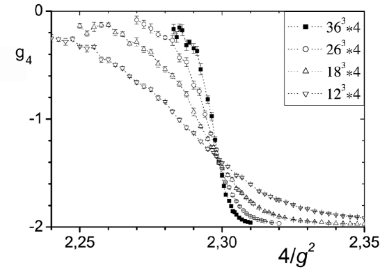
Figure 1: The fourth Binder cumulant $g_{4}$ on the lattices $N_{\tau}=4$; $N_{\sigma}=12,18,26,36$. MC data are taken from [5].

The results of the calculation of beta-function according to formula (24) are presented in Fig. 2 for three sets $N_{\sigma}=12$, $N^{\prime}_{\sigma}=18$; $N_{\sigma}=18$, $N^{\prime}_{\sigma}=26$; $N_{\sigma}=26$, $N^{\prime}_{\sigma}=36$. Although $N_{\sigma}$ and $N^{\prime}_{\sigma}$ in the different pairs are not too close, one can see surprisingly the coincidence of the curves at $4/g^{2}\geq 4/g_{c}^{2}$. This observation gives the hope that beta-function does not depend on the spatial size of lattice in the deconfinement phase.

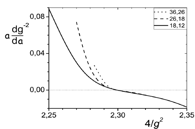
Figure 2: Beta-function from (24) for the pairs $N_{\sigma}=12$, $N^{\prime}_{\sigma}=18$; $N_{\sigma}=18$, $N^{\prime}_{\sigma}=26$; $N_{\sigma}=26$, $N^{\prime}_{\sigma}=36$.

Next we consider fixed $y=N_{\sigma}/N_{\tau}$, by varying $N_{\sigma}$, and therefore $N_{\tau}$ accordingly as is needed to reach the continuum limit. Rescaling $N_{\sigma}$ and $N_{\tau}$ by a factor $b$ leads to a phenomenological renormalization by the following identity for a scaling function $Q$

$$Q\Biggl{(}g_{t}\left(g^{-2},N_{\tau}\right)\cdot\left({N_{\sigma}\over N_{\tau}}\right)^{1/\nu}\Biggr{)}=Q\Biggl{(}g_{t}\left((g^{\prime})^{-2},N_{\tau}/b\right)\cdot\left({bN_{\sigma}\over bN_{\tau}}\right)^{1/\nu}\Biggr{)},$$ (25)

where $g_{t}(g^{-2},N_{\sigma})$ is determined by (12). If we ignore the possible $N_{\tau}$ dependence of the coefficients $c_{t}$ and $b_{t}$, then it follows from (25)

$$t\left(g^{-2},N_{\tau}\right)=t\left((g^{\prime})^{-2},N_{\tau}/b\right).$$ (26)

In general the reduced temperature $t=(T-T_{c})/T_{c}$ is a complicated function of the coupling $\beta=2N/g^{2}$, which in the vicinity of the critical temperature $T_{c}$ can be approximated by [2]

$$t=(\beta-\beta_{c}){1\over 4Nb_{0}}\left[1-{2Nb_{1}\over b_{0}}\beta_{c}^{-1}\right].$$ (27)

This approximation reproduces the correct reduced temperature in the continuum limit, which is easy verified by using (4). Taking the derivatives with respect to the scale parameter $b$ of the both sides of (26) and using (20) and (27) it is easy to obtain the expression for the beta-function

$$\beta_{f}(g)=-B_{0}(N_{\tau})g^{3}-B_{1}(N_{\tau})g^{5},$$ (28)

where

$$\left\{\begin{array}[]{l}B_{0}(N_{\tau})={\displaystyle 1\over\displaystyle 4N}\left(1-{\displaystyle 2Nb_{1}\over\displaystyle b_{0}\beta_{c}}\right){\displaystyle d\beta_{c}\over\displaystyle d\ln N_{\tau}}\\[8.5359pt] B_{1}(N_{\tau})=B_{0}(N_{\tau}){\displaystyle b_{1}\over\displaystyle b_{0}}.\end{array}\right.$$ (29)

Then the equation (2) leads to

$$a\Lambda_{{L}}=\exp\left(-{1\over 2B_{0}g^{2}}\right)\left(B_{0}g^{2}\right)^{-B_{1}/2B_{0}^{2}}.$$ (30)

Using (1) one can obtain the critical temperature $T_{c}$. The problem only remains to calculate the derivative $d\beta_{c}/d\ln N_{\tau}$ in expression (29). The calculation has been made for the SU(2) gauge theory by fitting the MC data for critical couplings $\beta_{c}^{{\rm MC}}(N_{\tau})$ with a spline interpolation and numerical differentiation of this curve. The result of the calculation is presented in Table 1. In comparison to $T_{c}/\lambda_{{L}}^{{\rm AF}}$ the much weaker dependence on $N_{\tau}$ of the critical temperature $T_{c}/\Lambda_{{L}}$ is observed.

$N_{\tau}$	$\beta_{c}=4/g_{c}^{2}$	$T_{c}/\Lambda_{{L}}^{{\rm AF}}$	$d\beta_{c}/dN_{\tau}$	$T_{c}/\Lambda_{{L}}$
2	1.880	29.7	–	–
3	2.177	41.4	0.158	25.22
4	2.299	42.1	0.086	25.46
5	2.373	40.6	0.063	25.38
6	2.427	38.7	0.045	24.13
8	2.512	36.0	0.040	24.24
16	2.739	32.0	0.017	–

Table 1: MC data for $\beta_{c}$ are taken from [2]. The values of $T_{c}/\Lambda_{{L}}^{{\rm AF}}$ are calculated from (4). Our results for $T_{c}/\Lambda_{{L}}$ are obtained from (30).

References

[1]
M. Creutz, Phys. Rev. D21 (1980) 2308.
[2]
J. Fingberg, V. Heller, and F. Karsch, Nucl. Phys. B392 (1993)
493.
[3]
J. Engels, F. Karsch, and K. Redlich, Nucl. Phys. B435 (1995)
295.
[4]
M.N. Barber, In: “Phase Transition and Critical Phenomena”, vol.
8, ed. C. Domb and J. Lebowitz (Academic Press, New York, 1981).
[5]
J. Engels, and T. Scheideler, Nucl. Phys. B539 (1999) 557.