Hedgehogs in Wilson loops and phase transition in SU(2) Yang-Mills theory

Abstract

We suggest that the gauge-invariant hedgehoglike structures in the Wilson loops are physically interesting degrees of freedom in the Yang–Mills theory. The trajectories of these “hedgehog loops” are closed curves corresponding to center-valued (untraced) Wilson loops and are characterized by the center charge and winding number. We show numerically in the SU(2) Yang–Mills theory that the density of hedgehog structures in the thermal Wilson–Polyakov line is very sensitive to the finite-temperature phase transition. The (additively normalized) hedgehog line density behaves like an order parameter: the density is almost independent of the temperature in the confinement phase and changes substantially as the system enters the deconfinement phase. In particular, our results suggest that the (static) hedgehog lines may be relevant degrees of freedom around the deconfinement transition and thus affect evolution of the quark-gluon plasma in high-energy heavy-ion collisions.

1 Introduction

Topological structures in fields are as important as the fields themselves. The well-known realization of this statement is the three-dimensional Georgi–Glashow (GG) model, which has topological defects called ’t Hooft–Polyakov (HP) monopoles [1]. The presence of these defects determine special features of the vacuum structure [2]: external electrically charged particles show linear confinement at large separations while the magnetic fields are screened at large distances. Neither the confinement nor the mass-gap generation are realized if the monopoles are absent in the vacuum (like, for example, in a case of the noncompact Abelian gauge theory).

Another textbook example is conventional superconductivity: in the Ginzburg–Landau approach the density of the superconducting electrons is described by the order-parameter field corresponding to an effective field of paired electrons (Cooper pairs). The topological structure in the Cooper-pair field is the Abrikosov vortex, which drastically influences the conduction and thermodynamic properties of conventional superconductors (for example, subjected to an external magnetic field).

The concept of topological defects in fields was invoked to understand color confinement. This phenomenon, which is one of the most interesting issues in QCD, is governed by gluons dynamics described by the pure Yang–Mills (YM) theory. The YM theories have zero-dimensional topological objects (instantons), but these objects cannot explain the color confinement [3] similarly to the GG model [2]. On the other hand, the YM theories lack topologically stable monopole-like and vortexlike classical configurations. Nevertheless, the confinement was suggested to be driven by condensation or, equivalently, by proliferation of the vortexlike [4] and monopole-like [5] nonclassical structures. Unfortunately, these structures alone are not supported topologically by the $SU(N)$ color symmetry of the YM theory in the continuum space–time. Therefore, the current understanding of color confinement is still unsatisfactory.

On the other hand, YM theory can be entirely formulated [6] in the language of colorless composite fields (Wilson loops), which are traces of the loop functionals of the gluon fields. Mathematically, these loops are as good as the gauge fields from the standpoint of describing properties (in particular, nonperturbative) of YM theories [6]. Having the importance of the order-parameter (Cooper-pair) field in the Ginzburg–Landau model of superconductivity in mind, we compare the properties of this field with the well-known properties of the Wilson loop variable in YM theory:

• Expectation values: The expectation value of the Cooper-pair field corresponds to the density of superconducting electrons, while the vacuum expectation value of the Wilson loop in YM theory is related to the interquark interaction. Both expectation values are order parameters (nonlocal in the case of the Wilson loop): the superconducting phase in ordinary superconductors is determined by a nonzero value of the Cooper-pair field, while the confining phase in the YM theories is manifested by an area-like asymptotic behavior of the Wilson loop.

• Correlation functions: The correlation function of the Cooper-pair fields determines the type and spectrum of the superconducting medium, while correlators of the Wilson loops provide information about the glueball spectrum of the strongly interacting medium, the intermeson interactions, etc.

• Topology: the topological structure in the Cooper-pair field is the celebrated Abrikosov vortex. What is an analog of this structure in the gluon fields of YM theory in the language of the Wilson loop variable? The answer to this question may be important for understanding color confinement because the Wilson loop operator itself is intimately related to this important phenomenon. Moreover, the mentioned structure in the Wilson loop must be a gauge-invariant quantity like the confinement phenomenon.

General arguments were given in [7] to identify the defect-like trajectories in the Yang-Mills theory with the closed paths in space for which the (untraced) Wilson loop takes its value in the center of the color group. The main argument in [7] is that the gluon fields in the vicinity of such “extremal” loops are similar to the gauge-invariant hedgehoglike structures, which resemble the HP monopoles in the GG model. Below we refer to these structures as to the “hedgehog loops”. Developing the idea further, we here investigate properties of the hedgehogs loops at a finite temperature. In particular, the static (thermal) hedgehoglike structures – which are also called below as the “hedgehog lines” – should definitely arise in an effective theory of Polyakov lines [8], which is proposed to describe basic features of the finite-temperature QCD transition. Moreover, the thermalization properties of the Polyakov line “condensate” [8] give a qualitatively encouraging insight regarding particle production in high-energy heavy-ion collisions [9]. As we show below, the density of the hedgehog lines in the deconfinement phase increases rapidly as temperature increases. This observation suggests that the hedgehog lines, corresponding to the extremal values in the Polyakov line variables, may be important degrees of freedom in quark-gluon states created in high-energy heavy-ion collisions.

The content of this paper is as follows. In Sec. 2, we define the hedgehog structure in the Wilson loop. Section 3 is devoted to a general discussion of hedgehog loop properties. In Sec. 4, we derive an expression for the density of the static hedgehogs (the hedgehog lines) as a function of the trace of the Polyakov line. We present the results of our numerical simulations in Sec. 5 and state conclusions in the last section.

2 Center-valued Wilson loops as hedgehog loops

The hedgehogs in the Wilson loops are similar to the HP monopoles in the GG model [7]. In this model the triplet Higgs field $\hat{\Phi}\equiv\frac{1}{2}\Phi^{a}\sigma^{a}$ of the static HP monopoles  [1] vanishes at the center of the HP monopole ${\mathbf{x}}={\mathbf{x}}_{0}$,

$$\hat{\Phi}({\mathbf{x}}_{0}) = 0\,.$$ (1)

Moreover, in spatial vicinity of a HP monopole the Higgs field has a generic hedgehog structure in the in a gauge where the gauge field $A_{\mu}$ is regular :

$$\hat{\Phi}({\mathbf{x}}) = \frac{\sigma^{a}}{2}Y^{ai}(x_{0})\cdot(x-x_{0})^{i}+O\Bigl{(}({\mathbf{x}}-{\mathbf{x}}_{0})^{2}\Bigr{)}\,.$$ (2)

Hedgehog structure (2) inevitably implies that Higgs field (1) vanishes, while the converse is false in general case. On the other hand, if the triplet field $\Phi$ vanishes at the point ${\mathbf{x}}_{0}$, then a general Taylor expansion of the field in the vicinity of this point starts from linear terms, and expansion (2) therefore corresponds to a generic situation. Note that the matrix $Y$ is assumed to be nondegenerate in a general case,

$${\mathrm{det}}\,Y\neq 0\,.$$

In YM theory,a hedgehog structure can be entirely defined in terms of Wilson-loop variables [7]. We consider an untraced Wilson loop beginning and ending at the point $x_{0}$ on the closed loop ${\mathcal{C}}$,

$$W_{\mathcal{C}}(x_{0})=P\,\exp\Bigl{\{}ig\,\oint_{{\mathcal{C}}}{\mathrm{d}}x_{\mu}\,A_{\mu}(x)\Bigr{\}}\,.$$ (3)

This quantity transforms locally as an adjoint operator with respect to the SU(2) color symmetry, $W_{\mathcal{C}}({\mathbf{x}}_{0})\to\Omega^{\dagger}({\mathbf{x}}_{0})W_{\mathcal{C}}({\mathbf{x}}_{0})\Omega({\mathbf{x}}_{0})$. To improve the analogy with the triplet Higgs field $\hat{\Phi}$, we subtract the singlet part from (3)

$$\hat{\Gamma}_{\mathcal{C}}(x_{0})=W_{\mathcal{C}}(x_{0})-{\mathchoice{\rm 1\mskip-4.0mul}{\rm 1\mskip-4.0mul}{\rm 1\mskip-4.5mul}{\rm 1\mskip-5.0mul}}\cdot\frac{1}{2}\,{\mathrm{Tr}}\,W_{\mathcal{C}}(x_{0})\,.$$ (4)

This is a traceless adjoint operator similar to the field $\hat{\Phi}$.

The next step is to associate the triplet part $\hat{\Gamma}_{\mathcal{C}}$ of Wilson loop (4) with the triplet Higgs field $\hat{\Phi}(x)$ in the GG model. To uncover a link between the hedgehog structures in the fields of the GG model and in the extremal loops of the YM theory, we notice the following [7]:

1. The Higgs field vanishes in all points $x$ belonging to the HP monopole trajectory, Eq. (1). Similarly, one could expect that the Wilson loop evaluated on the hedgehog loop ${\mathcal{C}}$ belongs to the center of the gauge group, $W_{\mathcal{C}}=\pm{\mathchoice{\rm 1\mskip-4.0mul}{\rm 1\mskip-4.0mul}{\rm 1\mskip-4.5mul}{\rm 1\mskip-5.0mul}}$. In turn, this implies that $\Gamma_{\mathcal{C}}$ vanishes on the hedgehog loop ${\mathcal{C}}$:

   $$W_{\mathcal{C}}\in{\mathbb{Z}}_{2}\qquad\Leftrightarrow\qquad\Gamma_{\mathcal{C}}=0\,.$$ (5)

   We intentionally omit the argument $x_{0}$ in the loop variables in Eq. (5) because condition (5) turns out to be independent of the choice of the reference point $x_{0}$ on the trajectory ${\mathcal{C}}$ [7]. In other words, if $W_{\mathcal{C}}(x_{1})\in{\mathbb{Z}}_{2}$ for at least one point $x_{1}\in{\mathcal{C}}$, then $W_{\mathcal{C}}(x_{0})\in{\mathbb{Z}}_{2}$ for all points $x_{0}\in{\mathcal{C}}$. This relation reflects self-consistency of our definition of the hedgehog loop.

   In order to illustrate the self-consistency, let us consider two Wilson loops lying on the same contour ${\mathcal{C}}$ but open at two different points $x_{0}$ and $x_{1}$. Both points are arbitrary. Then the corresponding Wilson loops (3) are related to each other by the adjoint transformation:

   $$W_{\mathcal{C}}(x_{1})=U^{\dagger}(x_{1},x_{0})\,W_{\mathcal{C}}(x_{0})\,U(x_{1},x_{0})\,,$$

   with

   $$U(x_{1},x_{0})=P\,\exp\Bigl{\{}ig\,\oint^{x_{1}}_{x_{0}}{\mathrm{d}}x_{\mu}\,A_{\mu}(x)\Bigr{\}}\in SU(2)\,.$$

   Obviously, if $W_{{\mathcal{C}}}(x_{0})\in{Z\!\!\!Z}_{2}$ then $W_{{\mathcal{C}}}(x_{1})\in{Z\!\!\!Z}_{2}$ as well, and, consequently, $\Gamma_{{\mathcal{C}}}(x_{1})\equiv 0$. Thus the condition (5) is insensitive to the reference point $x_{0}$.

   One can alternatively state that the independence of the definition of the hedgehog on the reference point $x_{0}$ manifests a conservation of the central charge $z$, which is defined in point iv below.

2. The triplet fields around the HP monopole have the structure of hedgehog (2). To demonstrate that the center-valued Wilson loop variables have something to do with the hedgehog structure, we infinitesimally deform the contour ${\mathcal{C}}\to{\mathcal{C}}+\delta{\mathcal{C}}$ in the vicinity of the point $x_{0}$. This shift also relocates the reference point, $x_{0}\to x=x_{0}+\delta x$ (see Fig. 1).

   
   

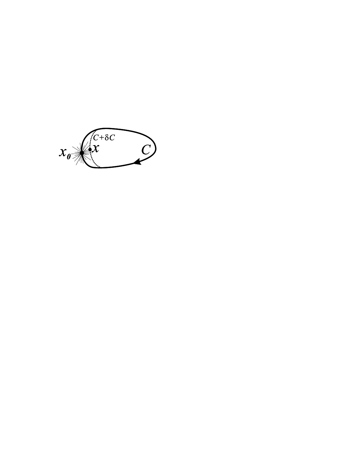
   Figure 1: The Wilson loop ${\mathcal{C}}$ (solid line) and its variation (dotted line).

   Without loss of generality, we assume that a tangent vector to the loop ${\mathcal{C}}$ at the point $x_{0}$ is aimed in the time direction. A physically distinguishable shift $\delta x$ should be tangential (spacelike) to the contour ${\mathcal{C}}$ because longitudinal (timelike) shifts of the point $x_{0}$ leave the functional $\Gamma_{\mathcal{C}}$ invariant.

   Then the deformed loop $\Gamma_{\mathcal{C}}(x)$, in general case, should have a spatial hedgehoglike structure in the vicinity of the zero point $x_{0}$,

   $$\Gamma_{\mathcal{C}}(x)=\frac{\sigma^{a}}{2}\,{\mathcal{Y}}^{ai}_{\mathcal{C}}(x_{0})\cdot{\bigl{(}x-x_{0}\bigr{)}}^{i}+O\Bigl{(}\bigl{(}x-x_{0}\bigr{)}^{2}\Bigr{)}\,.$$ (6)

   This structure is similar to that of Eq. (2) with only one exception: the definition of the matrix ${\mathcal{Y}}_{\mathcal{C}}$ involves the path derivative instead of the usual derivative,

   $${\mathcal{Y}}^{ai}_{\mathcal{C}}(x)=\frac{\delta\Gamma_{\mathcal{C}}^{a}(x)}{\delta x^{i}}{\Biggl{|}}_{x\to x_{0}}\,,\qquad a,i=1,2,3\,.$$ (7)

   which defines a change of the functional $\Gamma_{\mathcal{C}}$ under an infinitesimal change of the contour ${\mathcal{C}}\to{\mathcal{C}}+\delta C$.

   It is worth stressing that a loop at which the Wilson loop takes its value in the center of the gauge group correspond, in general case, to a hedgehog loop. This statement may not be true in a degenerate case, ${\mathrm{det}}{\mathcal{Y}}^{ai}_{\mathcal{C}}(x)=0$, which is realized, for example, in a trivial vacuum, $A^{a}_{\mu}=0$. The degenerate case is nongeneric and thus is statistically suppressed.

   Note that the matrix (7) can also be written in a explicitly Lorentz–invariant form,

   $${\mathcal{Y}}^{a\nu}_{\mathcal{C}}(x)\propto m^{\mu}_{\mathcal{C}}\,F^{a}_{\mu\nu}\,,$$

   where $m^{\mu}_{\mathcal{Y}}(x)=\dot{x}^{\mu}_{\mathcal{Y}}/|\dot{x}_{\mathcal{Y}}|$ is a vector which is tangent to the contour ${\mathcal{Y}}$ at the point $x$. The contour ${\mathcal{Y}}$ is parameterized by the vector function ${\bar{x}}^{\mu}_{\mathcal{Y}}$ of the variable $\tau$ and $\dot{x}^{\mu}_{\mathcal{Y}}\equiv\partial{\bar{x}}^{\mu}_{\mathcal{Y}}(\tau)/\partial\tau$.

3. The location $x_{0}$ of the HP monopole is a gauge-invariant quantity. Similarly, the trajectory ${\mathcal{C}}$ of the hedgehog loop in the Wilson loop defined by condition (5) is gauge invariant because the Wilson loop eigenvalues are gauge invariant.

4. The $SU(2)$ HP monopoles are classified by the integer-valued winding number $n\in\pi_{2}(S^{2})\simeq{\mathbb{Z}}$ corresponding the number of times the vacuum manifold $S^{2}$ is covered by a single turn around the two-dimensional boundary $\partial D_{3}\simeq S^{2}$ of the three-dimensional volume $D_{3}$ containing the HP monopole. Hedgehog structure (2) with $Y^{ai}\propto\delta^{ai}$ corresponds to the $n{=}1$ HP monopole in the GG model. In YM theory, the hedgehog loop is classified by the pair of numbers $(z,n)$, where $z=\pm 1$ is the central element of the Wilson loop $W_{\mathcal{C}}\in Z_{2}$ determined by Eq. (5) and $n$ is the winding number associated with hedgehogs structure (6). Below, we call $z$ the “center charge” of the hedgehog loop. A hedgehog line, which is a particular case of a general YM hedgehog in a Wilson loop, is also classified by the two charges.

5. The gluonic fields around a static hedgehog (or, equivalently, a thermal hedgehog line) share similarity with a field of a monopole in the axial gauge studied in [10]. However, in general, the hedgehog singularity has something to do with electric fields rather than with the magnetic ones. Indeed in the case of a static trajectory the matrix ${\mathcal{Y}}^{a\nu}$ becomes equal to the chromoelectric field, $E^{a}_{i}\equiv F^{a}_{4i}$, as one can deduce from Eq. (7) by an explicit calculation.

6. Because the hedgehog loops are closed, the hedgehog charges must be conserved.

3 Hedgehog loops and color confinement

As noted in the introduction, a close relation between the hedgehog loops and the color confinement problem can be understood intuitively on general grounds because the vacuum expectation value of the Wilson loops recognizes the color confinement. The hedgehog loops, corresponding to the extremal-valued Wilson loops, should also be sensitive to the color confinement. In this section, we argue in support of this suggestion.

In conventional superconductivity, Abrikosov vortices are singularities in the superconducting condensate (i.e., in the Cooper-pair field). In the core of the Abrikosov vortices, the superconductivity is broken, and the normal metal state is restored. It is well known that the weaker the Cooper-pair condensate is, the lighter (less tense) the Abrikosov vortices are. As temperature increases, the condensate weakens, and nucleation of the vortices due to thermal fluctuations strengthens. Thus, the higher the temperature is, the denser the (thermal) vortex ensemble should be.

It can be expected in the YM theory that the density of hedgehog loops is also sensitive to the phase transition. In the Euclidean formulation of the field theory, the temperature direction of the system volume is compactified to a circle whose circumference is equal to the inverse temperature. The order parameter of the phase transition is the vacuum expectation value of the (trace of the) Polyakov line,

$$\hat{L}({\mathbf{x}})=P\,\exp\Bigl{\{}ig\,\oint\limits_{0}^{1/T}{\mathrm{d}}x_{4}\,A_{4}({\mathbf{x}},x_{4})\Bigr{\}}\,,$$ (8)

which is static Wilson loop (3) closed through the boundary of the compactified (temperature) direction (we here define $L\equiv\frac{1}{2}{\mathrm{Tr}}\hat{L}$). Functional (8), also called the thermal Wilson line, is a basic variable in an effective theory proposed in [8] to describe the properties of the finite-temperature QCD transition. In the confinement phase, the expectation value of the Polyakov line is zero, $\langle L\rangle\equiv e^{-TF_{q}}=0$, indicating that the free energy of a single quark becomes infinite, $F_{q}\to\infty$. In the deconfinement phase, the Polyakov line has a nonzero expectation value, $\langle L\rangle\neq 0$, and the quarks are no longer confined.

It can be expected that static hedgehog lines (i.e., objects corresponding to the hedgehog structures in the Polyakov lines) are sensitive to the phase transition because the Polyakov line is the order parameter of this transition. In fact, the following analogy between the Cooper-pair condensate and the Polyakov line can be established. Both quantities are the order parameters, and the singularities in the Cooper pair condensate and the extremal values of the Polyakov lines should therefore be physically relevant degrees of freedom in the corresponding theories. As we show in the following sections, this suggestion is indeed correct. We note that this analogy is only partial because the core of the Abrikosov vortex corresponds to the unbroken vacuum while the vacuum in the core of the hedgehog loop in the Yang-Mills theory is maximally broken.

The behavior of the static hedgehog lines can be found qualitatively using symmetry arguments. The confinement–deconfinement phase transition is accompanied by breaking the global center symmetry in the deconfinement phase. This center symmetry is realized in the case of the $SU(2)$ Yang–Mills theory by the transformations $L(x)\to z\,L(x)$, where the factor $z=\pm 1$ belongs to the center of the gauge group, $z\in{Z\!\!\!Z}_{2}$. In the confinement phase, the center symmetry is unbroken, and the effective potential on the Polyakov variable, $V_{\mathrm{eff}}(L)=b_{2}L^{2}/2+b_{4}L^{4}/4+\dots$ with $b_{2,4}>0$, has a minimum at the symmetric vacuum $\langle L\rangle=0$, which is far away from the central values $L_{\pm}=\pm 1$. Therefore, the density of the hedgehogs lines should be small in the confinement phase.

In the deconfinement phase, the center symmetry is broken by the vacuum, and (as the temperature passes the critical value $T=T_{c}$) the single minimum of the effective potential splits into two ground states, $L_{\min}=\pm\sqrt{-b_{2}/b_{4}}$ with $b_{2}<0$, one of which is picked up by the vacuum $\langle L\rangle$. As the temperature increases further, the vacuum state approaches one of the central values $L_{\min}\to L_{\pm}=\pm 1$. Therefore, we expect to observe an increase in the density of static hedgehog lines characterized by the central charge $z$ closest to the vacuum state $\langle L\rangle$. The density of static hedgehog lines with the larger value of $|\langle L\rangle-z|$ should decrease in the deconfinement phase. The density of such intolerable hedgehog lines for $T>T_{c}$ should be lower than the density in the confinement phase. It is clear that at the critical temperature, the hedgehog line density should split into two branches.

The qualitative behavior of the spatial Wilson loops is known to be rather insensitive to the deconfinement transition: the area law for the spatial Wilson loops is observed in both the confinement and deconfinement phases. Therefore, we do not expect a drastic change in the density of spatial hedgehog loops as the YM system goes through the phase transition.

4 Density of static hedgehog lines

To go beyond the qualitative analysis presented in the preceding section, we would like to simulate the YM theory on the lattice numerically. But we immediately notice that the definition of the hedgehog loop (see 5 and 6) is rather inconvenient from the standpoint of numerical simulations. Indeed, the trajectory of the hedgehog structure in the Wilson loops cannot be determined locally as can be done in the case of the Abrikosov vortices in the Ginzburg–Landau model of superconductivity or in the case of the HP monopoles in the GG model. To check whether a hedgehog loop passes through a particular point $x$ in the space–time for one particular gauge-field configuration, we should analyze the Wilson loops $W_{\mathcal{C}}$ corresponding to all closed loops ${\mathcal{C}}$ that pass through the point $x\ni{\mathcal{C}}$. Obviously, it is difficult to realize this definition in numerical simulations of the YM theory on the lattice.

But at a finite temperature, static hedgehog lines are the most interesting because their density should show a noticeable change (in contrast to the spatial hedgehog loops) at the phase transition. In a continuum limit, it is easy to check whether a static hedgehog line passes through the particular point $x$ of the space. For this, we should evaluate (untraced) Polyakov line (8) and then check whether it belongs to the center of the group. In the $SU(2)$ YM model, the normalized trace of the Polyakov line on a static hedgehog line should be equal to $\pm 1$. In this section, we derive an analytic expression for the (absolute value of the) density of a static hedgehog line as a function of the traced Polyakov line $\rho=\rho[L]$.

Before proceeding further, we point out that in the static limit, hedgehog lines are similar to Abelian monopoles in the Polyakov and the Axial Abelian gauges of the SU(2) YM theory [11, 10, 12]. Because the Abelian monopoles in the Abelian Polyakov gauge are always static in the continuum limit, they are not related to the confinement of static quarks, but they still may be responsible for the spatial string tension at high temperatures [13]. Moreover, such monopoles are related to the topological charge in the YM theory [10, 12]. The Polyakov-loop variable can also be used to find (static) monopole constituents in physically interesting topologically nontrivial configurations [14]. We note that the density of static hedgehog lines (as well as the Polyakov line expectation value) is dual in a sense to the Abelian monopole condensate because the density of the hedgehog lines is expected to be an order parameter of the finite-temperature phase transition while the monopole condensate is a disorder parameter [15].

4.1 Density of static hedgehog lines in continuum

In general, the untraced Polyakov line can be expanded in the quaternion basis:

$$\hat{L}({\mathbf{x}},x_{4})=L({\mathbf{x}})\cdot{\mathchoice{\rm 1\mskip-4.0mul}{\rm 1\mskip-4.0mul}{\rm 1\mskip-4.5mul}{\rm 1\mskip-5.0mul}}+i(\vec{\Gamma}({\mathbf{x}},x_{4})\cdot\vec{\sigma})\,,$$ (9)

where the singlet part of $L$ is independent of $x_{4}$ and the components of the vector $\vec{\Gamma}$ describe the gauge-variant triplet part. If a hedgehog line passes through the point ${\mathbf{x}}_{0}$, then $L({\mathbf{x}})=\pm 1$ and $\vec{\Gamma}({\mathbf{x}}_{0})=0$. Therefore, the triplet part in a neighborhood of the point $\vec{x}_{0}$ can be expanded as

$$\Gamma^{a}({\mathbf{x}})=Y^{ai}({\mathbf{x}}_{0})\cdot(x-x_{0})^{i}+O\Bigl{(}({\mathbf{x}}-{\mathbf{x}}_{0})^{2}\Bigr{)}\,,$$ (10)

where ${\mathrm{det}}\,Y^{ab}({\mathbf{x}}_{0})\neq 0$ in general case. We do not consider the rare degenerate case ${\mathrm{det}}\,Y^{ab}({\mathbf{x}}_{0})=0$ here. Therefore the density of the static hedgehog line corresponds to the density of the points, where the Polyakov line takes its value in the center of the group. We note that Eq. (10) is similar to Eqs. (2) and (6).

The density of the hedgehog lines is expressed as

$$\rho=\gamma\,\delta(\vec{\Gamma}^{2})\equiv\frac{\gamma}{2|\vec{\Gamma}|}\cdot\delta(|\vec{\Gamma}|)\,,$$ (11)

where $\gamma$ is an unknown factor to be determined below. Because the quantity $\vec{\Gamma}$ is dimensionless, the dimension of the factor $\gamma$ should be [$mass^{3}$].

Using the identity $\delta(r)={4\pi r^{2}}\delta^{(3)}(\vec{r})$ and Eq. (11), we obtain $\rho[L]=2\pi\gamma|\vec{\Gamma}|\,\delta^{(3)}(\vec{\Gamma})$. Integrating this identity in the infinitesimally small volume $v_{{\mathbf{x}}_{0}}$ with ${\mathbf{x}}_{0}\ni v_{{\mathbf{x}}_{0}}$ gives the self-consistency condition, which allows us to determine the factor $\gamma$ in Eq. (11):

$$1=\int\limits_{v_{{\mathbf{x}}_{0}}}{\mathrm{d}}{\mathbf{x}}\,\rho({\mathbf{x}})=2\pi\int\limits_{v_{{\mathbf{x}}_{0}}}{\mathrm{d}}{\mathbf{x}}\,\gamma({\mathbf{x}})|\vec{\Phi}({\mathbf{x}})|\delta^{(3)}(\vec{\Phi}({\mathbf{x}}))\,.$$ (12)

Changing the integration variables from ${\mathrm{d}}{\mathbf{x}}$ to ${\mathrm{d}}\vec{\Gamma}$, we obtain the Jacobian factor,

$${\mathrm{d}}{\mathbf{x}}=\frac{1}{|{\det\frac{\partial\Gamma^{a}}{\partial x^{b}}}|}\,{\mathrm{d}}\vec{\Gamma}=\frac{1}{|\det Y^{ab}({\mathbf{x}}_{0})|}\,{\mathrm{d}}\vec{\Gamma}\,.$$ (13)

Substituting Eq. (13) in Eq. (12), we obtain

$$\gamma=\frac{\det|Y^{ab}|}{2\pi|\vec{\Gamma}|}\equiv\frac{1}{4\pi\sqrt{2(1-L^{2})}}\,\sqrt{\det\frac{\partial^{2}L^{2}}{\partial x^{i}\partial x^{j}}}\,,$$ (14)

where we use the identity $|\vec{\Gamma}|=\sqrt{1-L^{2}}$ and the relation

$$\frac{\partial^{2}L^{2}({\mathbf{x}})}{\partial x^{i}\partial x^{j}}{\Bigl{|}}_{{\mathbf{x}}={\mathbf{x}}_{0}}=2\,Y^{ai}({\mathbf{x}}_{0})\,Y^{aj}({\mathbf{x}}_{0})\,,$$ (15)

which follows from Eq. (10). Noticing that ${\mathrm{det}}[2\,Y^{T}({\mathbf{x}}_{0})\,Y({\mathbf{x}}_{0})]\equiv 8({\mathrm{det}}Y)^{2}$, we obtain Eq. (14). Substituting Eq. (14) in Eq. (11), we finally write the expression for the monopole density:

$$\rho[L({\mathbf{x}})]=\frac{1}{16}\frac{1}{\sqrt{2(1-L^{2}({\mathbf{x}}))}}\,\sqrt{\det{\Bigl{|}\Bigl{|}\frac{\partial^{2}}{\partial x^{i}\partial x^{j}}L^{2}({\mathbf{x}})\Bigr{|}\Bigr{|}}_{i,j}}\,\delta\left(1-L^{2}({\mathbf{x}})\right)\,,$$ (16)

where $L({\mathbf{x}})$ is the Polyakov line evaluated at the point ${\mathbf{x}}$. The determinant is taken over the three spatial indices $i,j=1,2,3$.

There are three important properties of formula (16). First, this expression depends only on the singlet part (trace) of the Polyakov line and is independent on the triplet part.

Second, Eq. (16) corresponds to the absolute density of hedgehog lines with a particular value of the central charge $z$. As mentioned, the hedgehog lines are described by the winding number $n$ and the center charge $z$. Equation (16) treats hedgehog lines with $\pm n$ winding numbers on equal footing while discriminating between different center charges $z$. Knowledge of the absolute density is enough for our exploratory study reported below. The information about the sign of the hedgehog charge is given by the sign of the determinant of the matrix $Y$, which can be computed explicitly if the triplet part of the (untraced) Polyakov line is calculated.

Third, Eq. (16) treats the loop variations (7) as ordinary variations because the object of our interest is static by definition. Equation (16) can be generalized to the nonstatic case by properly treating the loop variation discussed in Sec. 2.

4.2 Density of static hedgehog lines on the lattice

The density of hedgehog lines in the continuum space–time is given by Eq. (16). To obtain the corresponding equation on the lattice, we discretize the double derivatives in Eq. (16) straightforwardly:

$$\frac{\partial^{2}}{\partial x^{\mu}\partial x^{\mu}}f({\mathbf{x}})\to\Delta_{\mu}\Delta_{\mu}\,f({\mathbf{x}}) = f({\mathbf{x}}-\hat{\mu})-2f({\mathbf{x}})+f({\mathbf{x}}+\hat{\mu})\,,$$ (17)

$$\frac{\partial^{2}}{\partial x^{\mu}\partial x^{\nu}}f({\mathbf{x}})\to\Delta_{\mu}\Delta_{\nu}\,f({\mathbf{x}}) = \frac{1}{4}\sum_{P_{\mu},P_{\nu}=\pm 1}P_{\mu}P_{\nu}\,f({\mathbf{x}}+P_{\mu}\cdot\hat{\mu}+P_{\nu}\cdot\hat{\nu})\,,$$ (18)

where no sum over $\mu$ in Eq. (17) is implied. An illustration of the double derivatives is provided in Fig. 2.

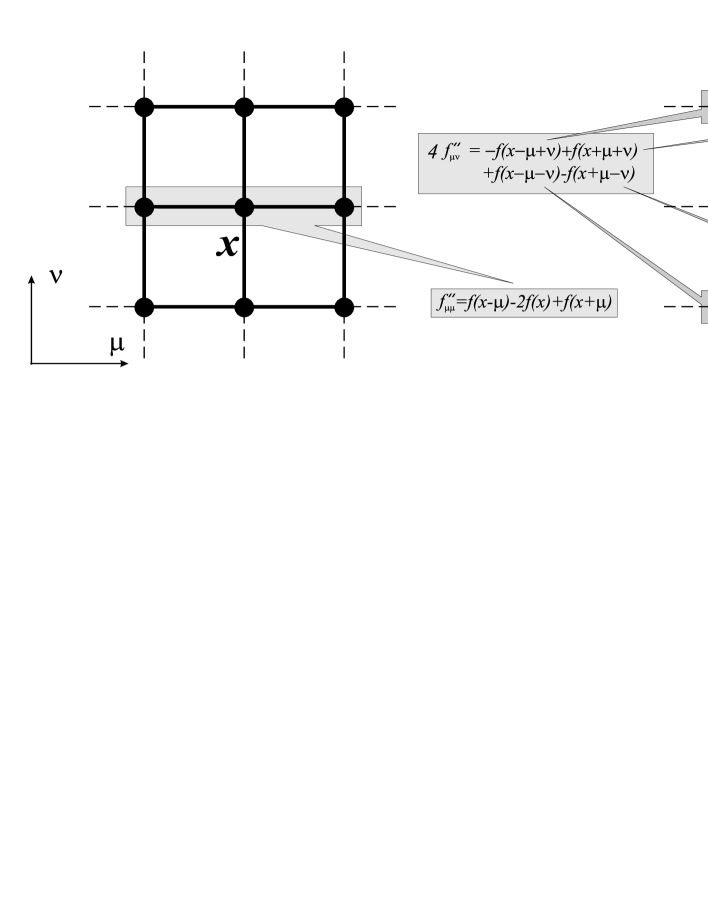
Figure 2: The lattice double derivatives $f^{\prime\prime}_{\mu\nu}({\mathbf{x}})\equiv\Delta_{\mu}\Delta_{\nu}\,f({\mathbf{x}})$ at the point ${\mathbf{x}}$.

The lattice version of density (16) can be expressed in the form

$$\rho\left[L({\mathbf{x}})\right]=\rho_{+}\left[L({\mathbf{x}})\right]+\rho_{-}\left[L({\mathbf{x}})\right]\,,$$ (19)

where the contributions of the positive and negative center loops to the total density can formally be written as

$$\rho_{\pm}\left[L({\mathbf{x}})\right]=d_{\pm}\left[L({\mathbf{x}})\right]\delta\Bigl{(}1\mp L({\mathbf{x}})\Bigr{)}\,.$$ (20)

The weights of the separate contributions of the positive and negative central loops are

$$d_{\pm}\left[L({\mathbf{x}})\right]=\frac{1}{64\,\sqrt{1\mp L({\mathbf{x}})}}\sqrt{\det{\Bigl{|}\Bigl{|}\Delta_{i}\Delta_{j}L^{2}({\mathbf{x}})\Bigr{|}\Bigr{|}}_{i,j}}\,,$$ (21)

Equation (20) is not suitable for use in the lattice simulations. From the practical standpoint, instead of Eq. (20) it is convenient to evaluate the distributions

$$\varrho_{\pm}(L_{0})=\left\langle d_{\pm}\left[L({\mathbf{x}})\right]\delta\Bigl{(}L_{0}-L({\mathbf{x}})\Bigr{)}\right\rangle\,.$$ (22)

Then the expectation values of monopole densities (19) are given by the limits

$$\langle\rho_{\pm}\rangle=\lim_{L_{0}\to\pm 1}\varrho_{\pm}(L_{0})\,.$$ (23)

5 Static hedgehog lines from lattice simulations

To investigate the static hedgehog lines numerically, we simulated the SU(2) gauge theory with the standard Wilson action on the asymmetric ($L_{s}^{3}\times L_{t}=20^{3}\times 4$) lattice with periodic boundary conditions in all directions. We used 100 independent configurations for each value of the gauge coupling, which ranges from $\beta=2.2$ to $\beta=2.5$. The SU(2) gauge theory has the second-order phase transition at $\beta\approx 2.30$ for this lattice geometry [17].

Before presenting the results for the center-valued loops, we first discuss some well-known properties of the Polyakov lines. The lattice Polyakov line is

$$P_{{\mathbf{x}}}[U]=\frac{1}{2}\,{\mathrm{T}r}\prod_{x_{4}=0}^{L_{t}-1}\,U_{4}({\mathbf{x}},x_{4})\,,$$ (24)

where $U_{x,\mu}$ is the lattice gauge field. The distribution of the Polyakov lines,

$$D(L)=\langle\delta(P_{{\mathbf{x}}}[U]-L)\rangle\,,$$ (25)

is symmetric in the confinement phase and asymmetric in the deconfinement phase in a sufficiently large system volume with periodic boundary conditions [16]. These properties reflect unbroken and broken ${Z\!\!\!Z}_{2}$ central symmetry, $L\to-L$, in the respective confinement and deconfinement phases.

Examples of typical distributions obtained for our gluon configurations are shown in Fig. 3.

(a)	(b)

Figure 3: Typical distributions (25) of Polyakov lines (24) in the confinement (a) and deconfinement (b) phases are shown by open circles. The filled circles correspond to $L\leftrightarrow-L$ symmetrized distributions.

We also show the distribution that is symmetrized under the discrete transformation $L\to-L$, which may be associated with jumps of the system from one ${Z\!\!\!Z}_{2}$ minimum to the other. In the deconfinement phase, the symmetric distribution has two maximums, which are known to become more pronounced as the volume of the system increases. These maximums in distributions correspond to minimums of the effective potential for the Polyakov variables discussed in Sec. 3.

In the confinement phase, the fluctuations of the Polyakov line are random and are therefore basically given by the symmetric Haar measure $D_{\mathrm{Haar}}(L){\mathrm{d}}L=(2/\pi)\sqrt{1-L^{2}}\,{\mathrm{d}}L$. In the deconfinement phase, the distribution is asymmetric and, consequently, far from flat. The distributions normalized by the Haar measure are shown in Fig. 4.

(a)	(b)

Figure 4: The same as in Fig. 3 but for normalized distributions ${\bar{D}}(L)=D(L)/\sqrt{1-L^{2}}$.

The qualitative behavior of the normalized distributions of the Polyakov line are very interesting to us because the Haar factor appears explicitly in the definition of density of the static hedgehog lines (16). The density of hedgehog lines thus explicitly excludes the effect of the Haar measure. The examples in Fig. 4 show that the normalized distribution of the Polyakov line is finite at the extremal end $L\to\pm 1$. To obtain an insight into the behavior of the extremal ends, we fit the Polyakov distributions by the simple linear function

$${\bar{D}}^{\mathrm{fit}}(L)=D_{z}+C_{z}(1-z\,L)\,,\quad\mbox{as}\quad L\to z=\pm 1\,,$$ (26)

where $D_{z}$ and $C_{z}$ are the fitting parameters labeled by the center element $z$. Examples of fits (26) are shown in Fig. 5.

(a)	(b)

Figure 5: Fits (26) of the normalized distributions ${\bar{D}}(L)=D(L)/\sqrt{1-L^{2}}$ in the confinement (a) and deconfinement (b) phases at both sides $L\to\pm 1$ of the distributions.

We also show the fits of the symmetrized distributions. As can be seen from these figures, the fits work very well. The extreme values of the distributions $D_{-1}\neq D_{+1}$ are clearly asymmetric in the deconfinement phase, $D_{\pm 1}\neq D_{\mathrm{sym}}\equiv\frac{1}{2}(D_{-1}+D_{+1})$ and are symmetric, $D_{\pm 1}=D_{\mathrm{sym}}$, in the confinement phase.

The extreme values $D_{z}$ of the normalized distributions $\bar{D}(L)$ are shown in Fig. 6(a)

(a)	(b)

Figure 6: (a) The extreme values $D_{z}$ of the normalized distributions of the Polyakov line. (b) The expectation value of the Polyakov line $|\langle L\rangle|$ as a function of the coupling $\beta$. The critical temperature $T_{c}$ corresponds to $\beta_{c}\approx 2.30$, and the deconfinement phase is realized at $\beta>\beta_{c}$ (equivalent to $T>T_{c}$).

as functions of the lattice coupling $\beta$. In the confinement phase ($\beta<\beta_{c}$), the quantities $D_{z}(\beta)$ are barely dependent on temperature ($\beta$). But as the temperature increases further, the system passes through the second-order phase transition, and the extreme quantities $D_{z}(\beta)$ with $z=\pm 1$ show a rapid change at the deconfinement point $\beta\approx\beta_{c}$. It can be clearly seen that the values $D_{-1}$ become enhanced while the quantity $D_{+1}$ becomes suppressed in the deconfinement phase. This corresponds the system residing in the $z=-1$ vacuum. For comparison, the expectation value of the Polyakov line as a function of $\beta$ is shown in Fig. 6(b).

Distributions (22) corresponding to the contributions $\varrho_{\pm}(L)$ of the negative and positive hedgehog lines (20) to total hedgehog line density (19) are shown in Fig. 7

(a)	(b)

Figure 7: Distributions (22) as functions of the Polyakov line $L$ in the confinement (a) and deconfinement (b) phases.

in the confinement and deconfinement phases. They indicate that the averaged quantities $\varrho_{\pm}(L)$ are not symmetric functions of $L$ both in the confinement and in the deconfinement phases: $\varrho_{\pm}(L)\neq\varrho_{\pm}(-L)$. This observation stresses the importance of $d_{\pm}$ factors (20) in the definition of the hedgehog line density. It can also be seen that the density distributions in the confinement phase are cross-symmetric in the sense that $\rho_{\pm}(L)=\varrho_{\mp}(-L)$. This cross-symmetry, which is a direct consequence of the ${\mathbb{Z}}_{2}$ center symmetry, is violated in the deconfinement phase.

Finally, the density of static hedgehog lines is given by the extreme values $L\to\pm 1$, Eq. (23), of distributions (22). To obtain these densities, we used a linear-fit function similar to Eq. (26). The densities $\rho_{-}$ and $\rho_{+}$ of the hedgehog lines with the respective center charges $z=-1$ and $z=+1$ are shown in Fig. 8

Figure 8: The densities $\rho_{z}$ of static hedgehogs corresponding to the positive and negative central charges $z=+1$ and $z=-1$ as a function of $\beta$. The vacuum resides at the negative center value $z=-1$. The dotted horizontal line marks the value $\rho_{\mathrm{conf}}$ of the densities in the confinement phase.

as a function of the gauge coupling $\beta$. A rapid increase in the density of $z{=}-1$ hedgehog lines, which correspond to the value of the center group closest the broken vacuum state, can be clearly observed. The hedgehog lines with the center charge $z=+1$ are far from the broken vacuum and are consequently suppressed in the infinitely high temperature limit. The symmetrized density, $\rho_{0}=\frac{1}{2}(\rho_{-}+\rho_{+})$, shows a less pronounced, but still noticeable, increase as the temperature increases in the deconfinement phase. In the confinement phase, all densities take the same value $\rho_{\mathrm{conf}}\approx{\mathrm{const}}$ and are independent of the temperature ($\beta$) within error bars. Our results thus indicate that the additively normalized density

$$\delta\rho_{z}(T)=\rho_{z}(T)-\rho(T=0)\,,\qquad z=\pm 1\,,$$ (27)

(as well as the corresponding symmetrized quantity $\delta\rho_{0}$) is an order parameter of the deconfinement phase transition.

Note that in the lattice units the density $\rho_{\pm}$ of the hedgehog lines - shown in Figure 8 – is more than by an order of magnitude smaller than the extreme values $D_{z}$ of the normalized distributions of the Polyakov line, Figure 6(a). The difference comes form the $d_{\pm}$ factors (21), which enter the definition of the density $\rho_{\pm}$ given in Eqs. (22) and (23).

We have also verified that the dependence of our results on the bin size of the distributions (shown in Fig. 7) is very weak. For example, at $\beta=2.33$ corresponding to the deconfinement phase, for one of the densities, the values $\rho_{+}=0.0427(17)$, $0.0455(29)$, and $0.0468(41)$, correspond to the respective bin numbers $N_{L}=100$, 200, and 300. A similar weak dependence on the number of bins is observed for $\rho_{-}$. The densities at other values of $\beta$ show the same behavior.

It is important to note the following. One could expect from the very beginning that the static hedgehog lines – being defined by the center elements of the gauge group – should be dense in the high-temperature phase since at very high temperatures the Polyakov line approaches a center element. However, this argument is not valid because, for example, it also leads to the erroneous conclusion that the hedgehog lines should be dense in the trivial vacuum, $A^{a}_{\mu}=0$. In fact, arguments of Ref. [7] indicate that the trivial vacuum does not possess the hedgehog lines at all. Technically, vanishing of the density of the hedgehog lines in the trivial vacuum is guaranteed by the determinant in Eq. (16). Thus, it is not clear ad hoc should the density of the hedgehog lines be high in the deconfinement phase or not. Consequently, the enhancement of the density of the hedgehog lines in the high temperature phase, Figure 8, is a non-trivial dynamical fact.

6 Conclusions

We have given analytic and numerical arguments supporting the suggestion [7] that the gauge-invariant hedgehoglike structures in Wilson loops (”the hedgehog loops”) are physically interesting degrees of freedom in Yang–Mills theory. The hedgehog loops can be defined self-consistently in terms of the Wilson loop variables. The hedgehog loops are associated with the (untraced) Wilson loops that take values in the center of the gauge group, $z\in{\mathbb{Z}}_{N}$. In the SU(2) Yang–Mills theory, the hedgehog loops are characterized by two quantized numbers: the center charge $z=\pm 1\in{\mathbb{Z}}_{2}$ and the winding number $n\in{\mathbb{Z}}$. Because the hedgehog loops are closed by construction, it seems natural to suggest that the corresponding charges $z$ and $n$ are conserved. In fact, the conservation of the center charge $z$ was proved in [7] and was discussed here. The conservation of the winding number $n$ along the hedgehog loop and a stability analysis of the hedgehog configurations in particular models may require an additional analysis.

From a general standpoint, it is clear that the hedgehog loops should be related to the confinement properties of the system because they are formulated in terms of the Wilson loops, which in turn are intimately related to color confinement in the Yang–Mills theory. The gauge invariance of hedgehog loops provides an additional argument in favor of their importance for gauge-invariant phenomena, like the color confinement. Unfortunately, the nonlocal formulation of the hedgehogs makes it difficult to locate these objects directly in separate configurations of the gluon fields. On the other hand, this difficulty can be circumvented by noticing that the statistical properties of hedgehogs can be studied using particular distributions corresponding to these objects with trajectories of predefined shapes. These distributions should provide information about densities, correlation properties, etc., of these objects.

In this paper, we have demonstrated the success of the proposed numerical approach by studying the properties of static hedgehog lines in the finite-temperature SU(2) gauge theory. By definition, static (or, ”thermal”) hedgehog line correspond to extremal (i.e., center) values of the Polyakov line variables, which should naturally arise in an effective model of the Polyakov lines [8]. This model is used to describe features of the finite-temperature QCD transition expected to be realized in the high-energy heavy-ion collisions [8, 9]. We showed numerically that the density of thermal hedgehogs changes rapidly as the temperature increases in the deconfinement phase. We observed a substantial increase (decrease) of the density of the thermal hedgehog lines with the central charge $z$ closest to (furthest from) the value of the Polyakov line in the centrally broken vacuum of the deconfinement phase. We thus found evidence that the hedgehog line density (additively normalized to zero at zero temperature) is an order parameter of the deconfinement phase transition. We conclude that hedgehogs in Wilson loops (in particular, in Polyakov lines) may be relevant degrees of freedom of the Yang–Mills vacuum.

References

- [1] G. ’t Hooft, Nucl. Phys. B 79 (1974) 276; A. M. Polyakov, JETP Lett. 20 (1974) 194; for a review see Yakov M. Shnir, “Magnetic Monopoles” (Springer, 2005).
- [2] A. M. Polyakov, Nucl. Phys. B 120 (1977) 429.
- [3] D. Diakonov, V. Y. Petrov, P. V. Pobylitsa, Phys. Lett. B 226 (1989) 372.
- [4] G. ’t Hooft, Nucl. Phys. B 153 (1979) 141; J. Ambjorn, P. Olesen, Nucl. Phys. B 170 (1980) 265; G. Mack, Phys. Rev. Lett. 45 (1980) 1378; J. Greensite, Prog. Part. Nucl. Phys. 51 (2003) 1.
- [5] Y. Nambu, Phys. Rev. D 10 (1974) 4262; S. Mandelstam, Phys. Rept. 23 (1976) 245; G. ’t Hooft, Nucl. Phys. B 190 (1981) 455.
- [6] S. Mandelstam, Phys. Rev. 175 (1968) 1580; K. G. Wilson, Phys. Rev. D 10 (1974) 2445; Y. Makeenko, A. A. Migdal, Nucl. Phys. B 188 (1981) 269.
- [7] M. N. Chernodub, Phys. Lett. 634 (2006) 255.
- [8] R. D. Pisarski, Phys. Rev. D 62 (2000) 111501(R).
- [9] A. Dumitru, R. D. Pisarski, Phys. Lett. B 504 (2001) 282.
- [10] O. Jahn, F. Lenz, Phys. Rev. D 58 (1998) 085006;
- [11] T. Suzuki, S. Ilyar, Y. Matsubara, T. Okude, K. Yotsuji, Phys. Lett. B 347 (1995) 375 [Erratum-ibid. B 351 (1995) 603]; S. Ejiri, S. i. Kitahara, Y. Matsubara, T. Okude, T. Suzuki, K. Yasuta, Nucl. Phys. Proc. Suppl. 47 (1996) 322; M. N. Chernodub, F. V. Gubarev, M. I. Polikarpov, A. I. Veselov, Prog. Theor. Phys. Suppl. 131 (1998) 309.
- [12] H. Reinhardt, Nucl. Phys. B 503 (1997) 505; C. Ford, U. G. Mitreuter, T. Tok, A. Wipf, J. M. Pawlowski, Annals Phys. 269 (1998) 26; O. Jahn, J. Phys. A 33 (2000) 2997.
- [13] M. N. Chernodub, Phys. Rev. D 69 (2004) 094504.
- [14] M. Garcia Perez, A. Gonzalez-Arroyo, A. Montero, P. van Baal, JHEP 9906 (1999) 001; F. Bruckmann, D. Nogradi, P. van Baal, Acta Phys. Polon. B 34 (2003) 5717; F. Bruckmann, E. M. Ilgenfritz, B. V. Martemyanov, P. van Baal, Phys. Rev. D 70 (2004) 105013.
- [15] M. N. Chernodub, M. I. Polikarpov, A. I. Veselov, Phys. Lett. B 399 (1997) 267; A. Di Giacomo, G. Paffuti, Phys. Rev. D 56 (1997) 6816; V. A. Belavin, M. N. Chernodub, M. I. Polikarpov, JETP Lett. 79 (2004) 245; Pis’ma v JETP 83 (2006) 367.
- [16] A. D. Kennedy, J. Kuti, S. Meyer and B. J. Pendleton, Phys. Rev. Lett. 54 (1985) 87.
- [17] J. Engels, J. Fingberg, M. Weber, Nucl. Phys. B 332 (1990) 737.
- [18] A. Gonzalez-Arroyo, “Yang–Mills fields on the 4-dimensional torus. (Classical theory)”, hep-th/9807108; A. Barresi, G. Burgio and M. Muller-Preussker, Nucl. Phys. Proc. Suppl. 119 (2003) 571; Phys. Rev. D 69 (2004) 094503; P. de Forcrand and O. Jahn, Nucl. Phys. B 651 (2003) 125.