Phase diagram at finite temperature and quark density
in the strong coupling limit of lattice QCD for color SU(3)

Abstract

We study the phase diagram of quark matter at finite temperature ($T$) and chemical potential ($\mu$) in the strong coupling limit of lattice QCD for color SU(3). We derive an analytical expression of the effective free energy as a function of $T$ and $\mu$, including baryon effects. The finite temperature effects are evaluated by integrating over the temporal link variable exactly in the Polyakov gauge with anti-periodic boundary condition for fermions. The obtained phase diagram shows the first and the second order phase transition at low and high temperatures, respectively, and those are separated by the tri-critical point in the chiral limit. Baryon has effects to reduce the effective free energy and to extend the hadron phase to a larger $\mu$ direction at low temperatures.

I Introduction

Exploring various phases of quark and nuclear matter has recently attracted much attention both theoretically and experimentally. In the Relativistic Heavy-Ion Collider (RHIC) experiments, it is probable that strongly interacting Quark Gluon Plasma is created in heavy-ion collisions QM2004 . The phase transition from hadron phase to QGP at high temperatures and at zero baryon chemical potential is predicted from lattice QCD LatticeReview ; Lattice05 , and various experimental signals at RHIC suggest the formation of QGP. On the other hand, compressed baryonic matter is created in heavy-ion collision experiments at lower energies, and cold and dense baryonic matter is realized in the core of neutron star. For these large baryon density matter, various interesting matter forms have been proposed so far. These states include admixture and superfluidity of hyperons and strange quarks in neutron star core hyperon , the ${}^{3}\mathrm{P}_{2}$ neutron superfluidity PTP:PionCondensation , pion pion ; PTP:PionCondensation and kaon kaon condensations, color ferromagnetic state ColorFerro , color superconductor (CSC) CSC , in addition to the formation of baryon rich QGP BaryonRichQGP:Nstar ; BaryonRichQGP:NNcollision .

The lattice QCD Monte-Carlo simulations are possible for hot baryon-free nuclear matter, and matter at small baryon density Muroya2003 ; LatticeFiniteMu can be studied by, for example, the Taylor expansion method around $\mu=0$ LatticeFiniteMu ; Taylor , analytic continuation method AC , canonical ensemble method Canonical and the improved reweighting method FodorKatz . However, properties of highly compressed matter are still under debate Lattice05 ; Taylor ; AC ; Canonical ; FodorKatz . This is because the fermion determinant, which is used as the weight in the Monte-Carlo simulation, becomes complex at finite chemical potential MuOnLattice ; FiniteMu:Problems . Thus, in order to attack the problem of compressed baryonic matter, it is necessary to invoke some approximations in QCD or to apply some effective models HatsudaKunihiro ; Fukushima2004 . A possible approach is to study color SU(2) QCD Muroya2003 ; Fukushima2004 ; SU2 ; Nishida2004a , where the fermion determinant is still a real number even at finite baryon chemical potential, but there are several essential differences between color SU(2) and SU(3) QCD. For example, the color anti-symmetric diquark pair becomes color singlet, whose nature would be very different from those discussed in the context of CSC, and this diquark pair is nothing but a baryon which is a boson in color SU(2) QCD.

One of the most instructive approximations to investigate the finite temperature $T$ and chemical potential $\mu$ of QCD is to consider the strong coupling limit of lattice QCD Kawamoto1981 ; KS1981 ; HKS1982 ; Kluberg-Stern ; DKS1984 ; DKS1986 ; DHK1985 ; Fukushima2004 ; SU2 ; Nishida2004a ; Azcoiti ; Ilgenfritz1985 ; Faldt1986 ; Bilic ; BilicCleymans ; Nishida2004b ; XQLuo ; MDP ; KawamotoShigemoto . In fact, effective free energy at finite $T$ of strong coupling lattice QCD was analytically derived and predicted the second order chiral symmetry restoration temperature DKS1984 ; DKS1986 . The strong coupling limit lattice QCD effective action for finite $\mu$ and zero temperature ($T=0$) was also derived with the help of lattice chemical potential MuOnLattice and predicted a phase transition near the density of baryonic formation DHK1985 . These investigations triggered many later analytic Fukushima2004 ; SU2 ; Nishida2004a ; Azcoiti ; Ilgenfritz1985 ; Faldt1986 ; Bilic ; BilicCleymans ; Nishida2004b ; XQLuo and semi-analytic MDP investigations of finite $T$ and $\mu$ of lattice QCD in the strong coupling. It is worth to mention that the Monte-Carlo numerical results of lattice QCD should reproduce the analytic result of the strong coupling, and the qualitative nature, and even quantitative nature for some physical values such as meson masses, are quite close to the reality of finite coupling results KS1981 ; KawamotoShigemoto .

Based on these past experiences, there have been recently renewed interests of strong coupling lattice QCD as an instructive guide to finite $T$ and $\mu$ QCD. The effective free energy of strong coupling limit of lattice QCD action for SU(2) was analytically derived in Nishida2004a . The effective free energy of finite $\mu$ and zero temperature ($T=0$) for SU(3) was derived by Azcoiti et al. Azcoiti , who developed a method to decompose the coupling term of the baryon and three quarks into the coupling terms of diquark auxiliary field ($\phi_{a}$) with two quarks and those of $\phi_{a}$ with a quark and a baryon. The effective free energy at finite $T$ and $\mu$ for SU(3) was obtained in Nishida2004b , but the baryon effects are ignored there. Thus there is no work which takes account of both finite temperature and baryon effects in the strong coupling limit of lattice QCD for color SU(3) yet.

In this paper, we study the phase diagram of quark matter at finite temperature ($T$) and finite chemical potential ($\mu$) in the strong coupling limit of lattice QCD for color SU(3). We derive an analytical expression of the effective free energy as a function of $T$ and $\mu$. We take account of both the mesonic and baryonic composite terms in the $1/d$ expansion of the lattice QCD action, and perform the temporal link variable ($U_{0}$) integral exactly in the Polyakov gauge with anti-periodic boundary condition for fermions, while we ignore the effects of finite diquark condensate. Firstly, our treatment is different from the works by Nishida Nishida2004b and Bilic et al. Bilic ; BilicCleymans , who extensively studied the phase diagram with the leading term in the $1/d$ expansion containing only the mesonic composites. Secondly, our formulation is different from the work by Azcoiti et al. Azcoiti , who made the one link integral also for $U_{0}$ which is an approximate treatment at finite temperatures. Thirdly, we propose a way to include the diquark condensate as a color singlet order parameter in Subsec. IV.4, although extensive study is not carried out and will be reported elsewhere.

This paper is organized as follows. In Sec. II, we derive an analytical expression of the effective free energy in the strong coupling limit of color SU(3) lattice QCD with finite temperature and quark chemical potential. In Sec. III, we study the phase diagram of strong coupling limit lattice QCD in the chiral limit. In Sec. IV, we examine the parameter dependence of the present model and compare our results with those in other treatments. Also we propose a formulation to include diquark condensates in a mean field ansatz. We stress the importance of baryon effects in the phase diagram. We summarize our results in Sec. V.

II Effective free energy in the strong coupling limit of lattice QCD

In this section, we derive an expression of the effective free energy in the strong coupling limit lattice QCD with $N_{c}=3$ with finite temperature and quark chemical potential in a mean field ansatz including the baryon effects. Chemical potential is introduced in the same way as in Ref. MuOnLattice . For the finite temperature treatment, we follow the work by Damgaard, Kawamoto and Shigemoto DKS1984 ; DKS1986 , in which the anti-periodic boundary condition for fermions is exactly treated and the integral over the temporal link variable $U_{0}$ is performed exactly in the Polyakov gauge. In order to apply this technique, we have to obtain the effective action in the bilinear form of the quark field. Such effective actions have been derived DKS1984 ; DKS1986 ; Ilgenfritz1985 ; Faldt1986 ; Bilic ; BilicCleymans ; Nishida2004b only with the leading order mesonic composite term in the $1/d$ expansion for color SU(3). We utilize the idea proposed by Azcoiti et al. Azcoiti to decompose the baryonic composite term. Throughout the paper, both of the temporal and spatial direction points on the lattice, $\beta=1/T$ and $L$, are assumed to be even integers, and the lattice spacing is set to be unity. While $T=1/\beta$ takes discrete values, the effective free energy is given as a function of $T$ (and $\mu$), then we consider $T$ as a continuous valued temperature.

II.1 Strong coupling limit and integral over spatial link variables

We start from an expression of lattice QCD action with one species of staggered fermion for color SU($N_{c}$). In the strong coupling limit ($g\to\infty$), we can ignore the pure gluonic part of the action, since it is proportional to $1/g^{2}$. As a result, the lattice action contains only those terms including fermions, $S_{F}$.

$$S_{F}[U,\chi,\bar{\chi}] = S_{F}^{(U_{0})}[U_{0},\chi,\bar{\chi}]$$ (1)

$$+ \sum_{j=1}^{d}S_{F}^{(U_{j})}[U_{j},\chi,\bar{\chi}]+S_{F}^{(m)}[\chi,\bar{\chi}]\ ,$$

$$S_{F}^{(U_{0})} = \frac{1}{2}\sum_{x}\left[\bar{\chi}(x)e^{\mu}U_{0}(x)\chi(x+\hat{0})\right.$$ (2)

$$~{}~{}~{}\left.-\bar{\chi}(x+\hat{0})e^{-\mu}U^{\dagger}_{0}(x)\chi(x)\right]\ ,$$

$$S_{F}^{(U_{j})} = \frac{1}{2}\sum_{x}\eta_{j}(x)\left[\bar{\chi}(x)U_{j}(x)\chi(x+\hat{j})\right.$$ (3)

$$~{}~{}~{}\left.-\bar{\chi}(x+\hat{j})U^{\dagger}_{j}(x)\chi(x)\right]\ ,$$

$$S_{F}^{(m)} = m_{0}\sum_{x}\bar{\chi}^{a}(x)\chi^{a}(x)\ ,$$ (4)

where we introduce the chemical potential $\mu$ in the same way to Ref. MuOnLattice . And $\eta_{j}(x)=(-1)^{x_{0}+x_{1}+\cdots+x_{j-1}},~{}(j=1,2,3)$ is a Kogut-Susskind factor. The staggered fermion $\chi$ represents the quark field, and the SU($N_{c}$) matrix $U_{\mu}$ represents the gauge link variable.

In the first step, we perform the group integral for spatial link variables, $U_{j}(x)$ ($j=1,2,3$). Integral of the leading and next-to-leading order terms in the $1/d$ expansion leads to the following action,

$$\int{\cal D}[U_{j}]e^{-\sum_{j=1}^{d}S_{F}^{(U_{j})}[U,\chi,\bar{\chi}]}\simeq e^{-S_{F}^{(j)}}\ ,$$ (5)

$$S_{F}^{(j)}[\chi^{a},\bar{\chi}^{a}]=-\frac{1}{2}(M,V_{M}M)-(\bar{B},V_{B}B)\ .$$ (6)

where the inner product of fields are defined as $(A,VB)\equiv\sum_{x,y}A(x)V(x,y)B(y)$. The mesonic and baryonic composites and their propagators are defined KS1981 ; HKS1982 as

$$M(x) = \bar{\chi}^{a}(x)\chi^{a}(x)\ ,$$ (7)

$$B(x) = {1\over N_{c}!}\varepsilon_{ab\cdots c}\chi^{a}(x)\chi^{b}(x)\cdots\chi^{c}(x)\ ,$$ (8)

$$\bar{B}(x) = {1\over N_{c}!}\varepsilon_{ab\cdots c}\bar{\chi}^{c}(x)\cdots\bar{\chi}^{b}(x)\bar{\chi}^{a}(x)\ ,$$ (9)

$$V_{M}(x,y) = {1\over 4N_{c}}\sum_{j=1}^{d}\left(\delta_{y,x+\hat{j}}+\delta_{y,x-\hat{j}}\right)\ ,$$ (10)

$$V_{B}(x,y) = (-1)^{N_{c}(N_{c}-1)/2}\sum_{j=1}^{d}\left\{\eta_{j}(x)\over 2\right\}^{N_{c}}$$ (11)

$$\times\left(\delta_{y,x+\hat{j}}+(-1)^{N_{c}}\delta_{y,x-\hat{j}}\right)\ .$$

Here we have utilized the SU($N_{c}$) group integral formulae,

$$\int d[U]U_{ab}U^{\dagger}_{cd}={1\over N_{c}}\delta_{ad}\delta_{bc}\ ,$$ (12)

$$\int d[U]U_{ab}U_{cd}\cdots U_{ef}={1\over N_{c}!}\varepsilon_{ac\cdots e}\varepsilon_{bd\cdots f}\ .$$ (13)

The baryonic composite action $(\bar{B},V_{B}B)$ is often ignored with $N_{c}\geq 3$, since it is proportional to $1/\sqrt{d^{N_{c}-2}}$ in the $1/d$ expansion Kluberg-Stern . This scaling can be understood as follows. Mesonic and baryonic propagators contains the sum over $j=1,2,\ldots d$, and they are considered to be proportional to $d$. In order to keep the mesonic term $(M,V_{M}M)/2$ finite in the large $d$ limit, the mesonic composite should be proportional to $d^{-1/2}$. Then the quark field, the baryonic composite, and the baryonic composite action are proportional to $d^{-1/4}$, $d^{-N_{c}/4}$, and $d^{-(N_{c}-2)/2}$, respectively. For the discussion of dense baryonic matter, however, we expect larger baryon effects. Thus we keep this baryonic composite action and proceed. In the following discussion, we consider $N_{c}=3$ case.

II.2 Auxiliary fields

The effective action Eq. (6) contains six fermion terms, while we have to obtain the effective action in the bilinear or pfaffian ZinnJustin form in $\chi$ to perform the quark field integral at finite temperature. In order to reduce the power in $\chi$ and $\bar{\chi}$, we introduce several auxiliary fields.

The highest power term $\bar{B}B$ containing six quarks can be reduced by introducing the auxiliary baryon field $b$ through the following identity,

$$e^{(\bar{B},V_{B}B)}=\mbox{det}V_{B}\int{\cal D}[\bar{b},b]e^{-(\bar{b},V_{B}^{-1}b)+(\bar{b},B)+(\bar{B},b)}\ .$$ (14)

Next, we decompose the coupling terms of the baryon and three quarks by using the technique developed in Azcoiti . We consider the following composite diquark field $D_{a}$.

$$D_{a}={\gamma\over 2}\varepsilon_{abc}\chi^{b}\chi^{c}+{1\over 3\gamma}\bar{\chi}^{a}b\ ,\quad D_{a}^{\dagger}={\gamma\over 2}\varepsilon_{abc}\bar{\chi}^{c}\bar{\chi}^{b}+{1\over 3\gamma}\bar{b}\chi^{a}\ .$$ (15)

These are the combinations of diquark and baryon-antiquark (antibaryon-quark) pairs, and have the color transformation properties of $\bar{\mathbb{3}}$ and $\mathbb{3}$ for $D_{a}$ and $D_{a}^{\dagger}$, respectively. The parameter $\gamma$ is introduced so as to generate the coupling terms, $\bar{B}b+\bar{b}B$.

$$D_{a}^{\dagger}D_{a} = \bar{B}b+\bar{b}B+Y\ ,$$ (16)

$$Y = {\gamma^{2}\over 2}M^{2}-{1\over 9\gamma^{2}}M\bar{b}b\ .$$ (17)

The decomposition in Ref. Azcoiti corresponds to $\gamma=2$. The product $D_{a}^{\dagger}D_{a}$ can be generated by the auxiliary field $\phi_{a}$, and we can replace $\bar{b}B+\bar{B}b$ terms as follows.

$$e^{\bar{b}B+\bar{B}b}=\int d[\phi_{a},\phi^{\dagger}_{a}]e^{-\phi_{a}^{\dagger}\phi_{a}+(\phi_{a}^{\dagger}D_{a}+D_{a}^{\dagger}\phi_{a})-Y}\ ,$$ (18)

where the expectation value of $\phi_{a}$ is the same as that for $D_{a}$, $\langle\phi_{a}\rangle=\langle{D_{a}}\rangle$.

In terms of the $1/d$ expansion, the baryonic auxiliary field $b$ is proportional to $d^{1/4}$, provided that the exponent in Eq. (14) is ${\cal O}(d^{-1/2})$. Thus the second term $\bar{\chi}b$ in $D_{a}$ is ${\cal O}(1)$, while the first term $\varepsilon_{abc}\chi^{b}\chi^{c}$ is proportional to $d^{-1/2}$, and we expect the dominance of the second term for large $d$. This may be the reason why we need the baryon-antiquark pair in discussing the diquark pair condensate.

In the next step, we decompose the coupling term of the baryon and mesonic composite, $M\bar{b}b$, by introducing the baryon potential auxiliary field $\omega$ though the identity,

$$e^{M\bar{b}b/9\gamma^{2}}=\int d[\omega]\,e^{-\omega^{2}/2-\omega(\alpha M+g_{\omega}\bar{b}b)-\alpha^{2}M^{2}/2}\ ,$$ (19)

where $g_{\omega}=1/9\alpha\gamma^{2}$ and $\langle{\omega}\rangle=-\langle{\alpha M+g_{\omega}\bar{b}{b}}\rangle$. Note that the local four baryon term becomes zero, $\bar{b}(x)b(x)\bar{b}(x)b(x)=0$, due to the Grassmann variable nature, which is a natural consequence of staggered fermion formulation for one-flavor.

Finally, we introduce the auxiliary field for chiral condensate. It is interesting to note that we have additional “mass” terms, $(\gamma^{2}+\alpha^{2})M^{2}/2$ for the mesonic composite $M$ through the decomposition of baryonic composite action by introducing the auxiliary diquark and baryon potential fields. These terms are made of four quarks, and it is not easy to handle in the quark integral. Therefore, we include these terms in the hopping term,

$$\frac{1}{2}(M,V_{M}M)-\frac{1}{2}(\gamma^{2}+\alpha^{2})M^{2}=\frac{1}{2}(M,\widetilde{V}_{M}M)\ ,$$ (20)

then it becomes possible to bosonize as,

$$e^{\frac{1}{2}(M,\widetilde{V}_{M}M)}=\int{\cal D}[\sigma]e^{-\frac{1}{2}(\sigma,\widetilde{V}_{M}\sigma)-(\sigma,\widetilde{V}_{M}M)}\ ,$$ (21)

$$\widetilde{V}_{M}(x,y)=V_{M}(x,y)-(\gamma^{2}+\alpha^{2})\delta_{x,y}\ .$$ (22)

The expectation value of $\sigma$ is given as $\langle{\sigma}\rangle=-\langle{M}\rangle$. The mesonic propagator $\widetilde{V}_{M}$ has negative eigenvalues as well as positive ones, and thus it is expected that instability is introduced in the gaussian integration. However in the mean field ansatz, vacuum expectation value of the meson is introduced so that next neighboring $(x,x+\hat{\mu})$ dependence is suppressed, which corresponds to the suppression of $(x,y)$ dependence in $\widetilde{V}_{M}(x,y)$. In this way, we circumvent the instability, which is done in the literature and we show in the following.

After these sequential introduction of auxiliary fields, we obtain the action of quarks, baryons, diquarks, baryon potential, and the chiral condensate as follows.

$$S_{F}=S_{F}^{(X)}+S_{F}^{(q)}\ ,$$ (23)

$$S_{F}^{(X)}[b,\bar{b},\phi,\phi^{\dagger},\sigma,\omega]$$

$$~{}=(\bar{b},\widetilde{V}_{B}^{-1}b)+(\phi^{\dagger},\phi)+\frac{1}{2}(\omega,\omega)+\frac{1}{2}(\sigma,\widetilde{V}_{M}\sigma)\ ,$$ (24)

$$S_{F}^{(q)}[U_{0},\chi,\bar{\chi},b,\bar{b},\phi,\phi^{\dagger},\sigma,\omega]$$

$$~{}=S_{F}^{U_{0}}+({m_{q}},M)+{1\over 3\gamma}\left[(\bar{\chi}^{a},\phi_{a}^{\dagger}b)+(\bar{b}\phi_{a},\chi^{a})\right]$$

$$~{}~{}~{}~{}+\frac{\gamma}{2}\varepsilon_{cab}\left[(\phi_{c}^{\dagger},\chi^{a}\chi^{b})+(\bar{\chi}^{b}\bar{\chi}^{a},\phi_{c})\right]\ ,$$ (25)

$${m_{q}}=\widetilde{V}_{M}\sigma+\alpha\omega+m_{0}\ .$$ (26)

where $S_{F}^{(X)}$ and $S_{F}^{(q)}$ are the action of pure auxiliary fields and the action containing quarks, respectively. The inverse baryonic propagator is modified as

$$\widetilde{V}_{B}^{-1}(x,y)=V_{B}^{-1}(x,y)+g_{\omega}\omega\delta_{x,y}\ ,\quad g_{\omega}={1\over 9\alpha\gamma^{2}}\ .$$ (27)

It is noteworthy that the quark action is decomposed into that for each spatial point, $\mathbb{x}$. Therefore, it would be good enough to assume that bosonic auxiliary fields have constant values, i.e. mean field ansatz would be valid. This simplifies the term containing $\widetilde{V}_{M}\sigma$ as follows,

$$\widetilde{V}_{M}\sigma=a_{\sigma}\sigma\ ,\quad\frac{1}{2}(\sigma,\widetilde{V}_{M}\sigma)=\frac{\beta L^{3}}{2}a_{\sigma}\sigma^{2}\ ,$$ (28)

$$a_{\sigma}={d\over 2N_{c}}-(\gamma^{2}+\alpha^{2})\ .$$ (29)

II.3 Quark integral

In order to perform the quark integral, we would like to separate the action into terms, each of which has as small number of quark fields as possible. In the quark action Eq. (25), the time component of the link variable $U_{0}$ connect the quark field of different (imaginary) time, and all the quark fields with different times couple.

This coupling is known to be separated by using the Fourier transformation for the fermion fields DKS1984 ; DKS1986 ,

$$\psi(x)={1\over\sqrt{\beta}}\sum_{m=1}^{\beta}e^{ik_{m}\tau}\psi_{m}(\mathbb{x})\ ,$$ (30)

$$\bar{\psi}(x)={1\over\sqrt{\beta}}\sum_{m=1}^{\beta}e^{-ik_{m}\tau}\bar{\psi}_{m}(\mathbb{x})\ ,$$ (31)

where $\psi$ stands for $\chi$ or $b$, and the Matsubara frequencies, $k_{m}=2\pi(m-1/2)/\beta$, are selected to satisfy anti-periodic condition of fermions, $\psi(\beta,\mathbb{x})=-\psi(0,\mathbb{x})$, to introduce temperature effects.

We ignore the time dependence of bosonic auxiliary fields, $\phi,\phi^{\dagger},\omega,\sigma$ (static approximation), and we work in the Polyakov gauge, where the link variable $U_{0}$ is diagonal and independent on time,

$$U_{0}(\mathbb{x},\tau)={\rm diag}(e^{i\theta_{1}(\mathbb{x})/\beta},e^{i\theta_{2}(\mathbb{x})/\beta},e^{i\theta_{3}(\mathbb{x})/\beta})\ ,$$ (32)

with the condition $\theta_{1}+\theta_{2}+\theta_{3}=0$. The quark action is found to be represented in the form of pfaffian,

$$S_{F}^{(q)} = \frac{1}{2}\sum_{\mathbb{x},m,n}(\bar{\chi}^{a}_{m},\chi^{a}_{m})\mathbb{G}^{-1}_{ab}(m,n)\begin{pmatrix}\chi^{b}_{n}\\ \bar{\chi}^{b}_{n}\\ \end{pmatrix}$$ (33)

$$+ \sum_{\mathbb{x},m}\left(\bar{C}^{a}_{m}\chi^{a}_{m}+\bar{\chi}^{a}_{m}C^{a}_{m}\right)\ ,$$

$$\mathbb{G}^{-1}_{ab}(m,n;\theta_{a})=\begin{pmatrix}B^{a}(k_{m})\delta_{ab}\delta_{mn}&-\gamma\varepsilon_{cab}\phi_{c}\delta^{\prime}_{mn}\\ \gamma\varepsilon_{cab}\phi_{c}^{\dagger}\delta^{\prime}_{mn}&-B^{a}(k_{m})\delta_{ab}\delta_{mn}\\ \end{pmatrix}\ ,$$ (34)

$$B^{a}(k)={m_{q}}+i\sin(k+\theta^{a}/\beta-i\mu)\ ,$$ (35)

$$C^{a}_{m}=\frac{1}{3\gamma}\phi_{a}^{\dagger}b_{m}\ ,\quad\bar{C}^{a}_{m}=\frac{1}{3\gamma}\bar{b}_{m}\phi_{a}\ .$$ (36)

In the first line of Eq. (33), we have used the notation $\delta^{\prime}_{mn}=\delta_{m,\beta-n+1}$. The second term in Eq. (33) can be absorbed into the first term by shifting the quark field at a cost of producing another term $S_{F}^{(C)}$, which is bilinear in $b$ and $\bar{b}$.

$$S_{F}^{(q)} = \frac{1}{2}\sum_{\mathbb{x},m,n}(\bar{\chi}^{a}_{m},\chi^{a}_{m})\mathbb{G}^{-1}_{ab}(m,n)\begin{pmatrix}\chi^{b}_{n}\\ \bar{\chi}^{b}_{n}\\ \end{pmatrix}+S_{F}^{(C)}\ ,$$ (37)

$$S_{F}^{(C)} = -\frac{1}{2}\sum_{\mathbb{x},m,n}(\bar{C}^{a}_{m},-C^{a}_{m})\mathbb{G}_{ab}(m,n)\begin{pmatrix}C^{b}_{n}\\ -\bar{C}^{b}_{n}\\ \end{pmatrix}\ .$$ (38)

The action $S_{F}^{(C)}$ appears from the baryon-quark coupling generated by the diquark condensate, and it is very difficult to handle with finite values of $\phi$. Another treatment to replace this coupling by other terms will be discussed in Subsec. IV.4, and we temporarily ignore $S_{F}^{(C)}$ here. In this case, by symmetrizing for $m$ and $m^{\prime}=\beta-m+1$ in Eq. (33), We obtain the block diagonal form of $S_{F}^{q}$,

$$S_{F}^{(q)}=\sum_{\mathbb{x},a,b}\sum_{m=1}^{\beta/2}(\bar{\chi}^{a}_{m},\chi^{a}_{m^{\prime}})\mathbb{g}_{ab}(k_{m})\begin{pmatrix}\chi^{b}_{m}\\ -\bar{\chi}^{b}_{m^{\prime}}\\ \end{pmatrix}\ .$$ (39)

$$\mathbb{g}_{ab}(k)=\begin{pmatrix}\mathbb{B}(k)_{ab}&\mathbb{A}_{ab}\\ \mathbb{A}_{ab}^{*}&\mathbb{B}(-k)_{ab}\\ \end{pmatrix}\ ,$$ (40)

Here, $(\mathbb{B}(k))_{ab}=\delta_{ab}B^{a}(k)$, $(\mathbb{A})_{ab}=\gamma\varepsilon_{cab}\phi_{c}$ and we have used the relation, $k_{m^{\prime}}=2\pi-k_{m}=-k_{m}({\rm mod}(2\pi))$. Since $\bar{\chi}_{m},~{}\chi_{m^{\prime}}$ are independent of each other, Grassmann integral over $\chi,\bar{\chi}$ leads to a determinant:

$$\int{\cal D}[\chi,\bar{\chi}]e^{-S_{F}^{(q)}}=\prod_{\mathbb{x}}G(\mathbb{x})\ .$$ (41)

$$G(\mathbb{x})\equiv\prod_{m=1}^{\beta/2}\mbox{det}\left[\mathbb{g}_{ab}(k_{m})\right]=\prod_{m=1}^{\beta}\mbox{det}\left[\mathbb{g}_{ab}(k_{m})\right]^{1/2}\ .$$ (42)

The $G(\mathbb{x})$ is evaluated by the direct calculation of $\det$:

$$G(\mathbb{x}) = \prod_{m=1}^{\beta/2}\Bigl{[}\gamma^{4}(B_{1}|\phi_{1}|^{2}+B_{2}|\phi_{2}|^{2}+B_{3}|\phi_{3}|^{2})$$ (43)

$$\times(B_{1}^{\prime}|\phi_{1}|^{2}+B_{2}^{\prime}|\phi_{2}|^{2}+B_{3}^{\prime}|\phi_{3}|^{2})$$

$$+ \gamma^{2}\sum_{(a,b,c)=cyc.}B_{a}B_{a}^{\prime}|\phi_{a}|^{2}(B_{b}B_{c}^{\prime}+B_{b}^{\prime}B_{c})$$

$$+ B_{1}B_{2}B_{3}B_{1}^{\prime}B_{2}^{\prime}B_{3}^{\prime}\Bigr{]}\ ,$$

where $B_{a}=B^{a}(k_{m}),B_{a}^{\prime}=B^{a}(-k_{m})$. In a similar way to that in Ref. Nishida2004a , we can perform the Matsubara frequency product $\prod_{m}$,

$$G(\mathbb{x})=\prod_{j}\bigl{[}1+e^{-i\beta z_{j}(\mathbb{x})}\bigr{]}^{1/2},$$ (44)

where $z_{j}(\mathbb{x})$ is the solution of $\mbox{det}\left[\mathbb{g}_{ab}(k_{m})\right]=0$. The explicit derivation is given in the Appendix A.

II.4 Effective free energy at zero diquark condensate

When the diquark condensate is zero, $\phi_{a}=0$, we know the solutions of $\mbox{det}\left[\mathbb{g}_{ab}(k_{m})\right]=0$. We can take $B_{a}=B^{a}(k)=0$ and $B_{a}^{\prime}=B^{a}(-k)=0$, and we get four solutions for each $a$,

$$i\beta z_{a}=\pm\left[i(\theta_{a}-i\beta\mu)\pm\beta{E_{q}}({m_{q}})\right]\ ,$$ (45)

where $E_{q}({m_{q}})=\mathrm{arcsinh}\,{m_{q}}$ is one dimensional quark excitation energy. We can then explicitly write the quark integral results as,

$$G(\mathbb{x}) = \prod_{a=1}^{N_{c}}\left[(1+e^{-i(\theta_{a}-i\beta\mu)-\beta{E_{q}}})(1+e^{-i(\theta_{a}-i\beta\mu)+\beta{E_{q}}})\right.$$ (46)

$$\times\left.(1+e^{i(\theta_{a}-i\beta\mu)-\beta{E_{q}}})(1+e^{i(\theta_{a}-i\beta\mu)+\beta{E_{q}}})\right]^{1/2}$$

$$= \prod_{a=1}^{N_{c}}2\left(\cos(\theta-i\beta\mu)+\cosh{E_{q}}\right)$$

$$= \prod_{a}2\left(C_{\sigma}+C_{\mu}\cos\theta_{a}+iS_{\mu}\sin\theta_{a}\right)\ ,$$

$$C_{\sigma} = \cosh\beta{E_{q}}\ ,\;C_{\mu}=\cosh\beta\mu\ ,\;S_{\mu}=\sinh\,\beta\mu\ .$$ (47)

There are three comments on the phase of $G(\mathbb{x})$ in order. First, the square root in the quark determinant (Eq. (44)) is the Pfaffian root ZinnJustin , but it comes from the square root in Eq. (42), where we extend the range of the Matsubara product from $\beta/2$ to $\beta$ by using the even function nature of $\mbox{det}\left[\mathbb{g}_{ab}(k_{m})\right]=\mbox{det}\left[\mathbb{g}_{ab}(-k_{m}=k_{m^{\prime}})\right]$. Since the phase of the square root in Eq. (42) is defined to reproduce the product up to $\beta/2$, there is no phase ambiguity. This is because we can represent the quark action $S_{F}^{(q)}$ in Eq. (39) in a usual bilinear fermion action by defining a new fermion field as $(\psi^{b}_{m^{\prime}},\bar{\psi}^{a}_{m^{\prime}})\equiv(-\bar{\chi}^{b}_{m^{\prime}},\chi^{a}_{m^{\prime}})$, then it is not necessary to introduce the Pfaffian root. Secondly, we may have a phase coming from a constant in $\log G(\mathbb{x})$ as shown in the Appendix A, but this constant does not depend on the gluon configurations $\theta_{a}(\mathbb{x})$. As a result, we have a fixed phase for a given spatial point $\mathbb{x}$, and we get well-defined integral of $G(\mathbb{x})$ over $dU_{0}(\mathbb{x})$. In this way, we expect that we get reasonable continuum limit, which we can still consider in the strong coupling region. Thirdly, in order to take one flavor fermion configuration, we have to take one quarter root of Eq. (46), where the well known phase ambiguity of complex number appears Golterman2006 . Here, we simply consider configuration with one species of staggered fermion, which in general regarded as four flavor configurations, and do not take into account the complexity of the four flavor feature of staggered fermion.

By using the SU(3) Haar measure in the Polyakov gauge,

$$\int dU_{0}(\mathbb{x})=\int{d\theta_{1}d\theta_{2}d\theta_{3}\over(2\pi)^{3}}\Delta(\theta_{1},\theta_{2},\theta_{3})\ ,$$ (48)

$$\Delta=\delta(\theta_{1}+\theta_{2}+\theta_{3})\prod_{i<j}(1-\cos(\theta_{i}-\theta_{j}))\ ,$$ (49)

the integral over $U_{0}$ can be performed analytically.

$$\exp\left(-\beta L^{3}F_{{\rm eff}}^{(q)}\right)\equiv\prod_{\mathbb{x}}\int dU_{0}(\mathbb{x})G(\mathbb{x})\ ,$$ (50)

$$F_{{\rm eff}}^{(q)}(\sigma)=-T\log\left[\frac{4}{3}\left(C_{\sigma}^{3}-\frac{1}{2}C_{\sigma}+\frac{1}{4}C_{N_{c}\mu}\right)\right]\ ,$$ (51)

$$C_{\sigma}=\cosh{{E_{q}}\over T}\ ,\quad C_{N_{c}\mu}=\cosh{N_{c}\mu\over T}\ .$$ (52)

where $T=1/\beta$ is regarded as a temperature. It is interesting to find that $G(\mathbb{x})$ can have a complex phase for a given gluon configuration, but after integration over the temporal link variables, we have a positive definite results and we do not have the sign problem. This is one of the merits in the strong coupling limit in which the link integral can be performed in an analytic manner. This result is consistent with that for SU($N_{c}$) shown in, for example, Ref. Nishida2004b ,

$$F_{{\rm eff}}^{(q)}=-T\log\left\{{\sinh[(N_{c}+1)E/T]\over\sinh[E/T]}+2C_{N_{c}\mu}\right\}\ ,$$ (53)

while $C_{N_{c}\mu}$ term does not appear in $\textrm{U}(N_{c})$ case DKS1984 ; DKS1986 .

When the diquark condensate is zero, $\phi_{a}=0$, we can ignore $S_{F}^{(C)}$, and it becomes possible to perform baryon integral, too:

$$F_{{\rm eff}}^{(b)}(g_{\omega}\omega)={1\over\beta L^{3}}\log{\rm Det}\left[1+g_{\omega}\omega V_{B}\right]\ .$$

As shown in the Appendix B, we can evaluate this determinant by using the Fourier transformation. For large spatial lattice size $L$, by replacing the sum over $\mathbb{k}$ by the integral, we get the following expression,

$$F_{{\rm eff}}^{(b)}(g_{\omega}\omega) \simeq \frac{-a^{(b)}_{0}/2}{\left(4\pi\Lambda^{3}/3\right)}\int_{0}^{\Lambda}4\pi k^{2}dk\log\left[1+{g_{\omega}^{2}\omega^{2}k^{2}\over 16}\right]$$ (54)

$$=-a_{0}^{(b)}f^{(b)}\left(\frac{g_{\omega}\omega\Lambda}{4}\right)\ ,$$

where, $a^{(b)}_{0}=1.0055\ ,~{}\Lambda=1.01502\times\pi/2$, and $f^{(b)}(x)$ is given as,

$$f^{(b)}(x)=\frac{1}{2}\log(1+x^{2})-{1\over x^{3}}\left[\arctan{x}-x+{x^{3}\over 3}\right]\ .$$ (55)

Since this baryon determinant term $F_{{\rm eff}}^{(b)}$ is independent from $T$ and $\mu$, it would be more convenient for the later discussion to separate the quadratic term in $\omega$ as follows,

$${\omega^{2}\over 2}+F_{{\rm eff}}^{(b)}(g_{\omega}\omega) = \frac{1}{2}a_{\omega}\omega^{2}+\Delta F_{{\rm eff}}^{(b)}(g_{\omega}\omega)\ ,$$ (56)

$$a_{\omega} = 1-{3\over 5}a_{0}^{(b)}\left({g_{\omega}\Lambda\over 4}\right)^{2}\ ,$$ (57)

where $\Delta F_{{\rm eff}}^{(b)}={\cal O}(\omega^{4})$ at small $\omega$ values. The second term in $a_{\omega}$ comes from the expansion of Eq.(54).

After quark, gluon and baryon integral, the total effective free energy is obtained as,

$${\cal F}_{{\rm eff}}=\frac{1}{2}a_{\sigma}\sigma^{2}+\frac{1}{2}a_{\omega}\omega^{2}+F_{{\rm eff}}^{(q)}({m_{q}})+\Delta F_{{\rm eff}}^{(b)}(g_{\omega}\omega)\ ,$$ (58)

where ${m_{q}}=a_{\sigma}\sigma+\alpha\omega+m_{0}$.

II.5 Stability and equilibrium condition

We have introduced two parameters, $\gamma$ and $\alpha$, and two auxiliary fields, $\sigma$ and $\omega$, in the derivation of the effective free energy, Eq. (58). Since we have introduced these parameters and fields through identities, the final results should not depend on these parameters if all the integrals are completed. However, we are working in the mean field ansatz, then we may have some parameter dependence. In principle, we should select the parameters so as to keep the mean field ansatz valid; the effective free energy should be stable against the variation of the fields, $\sigma$ and $\omega$, and the effective free energy (the free-energy density) at equilibrium should be stationary against the variation of parameters. We further require that the chiral symmetry is restored at very high temperatures. The stability of the effective free energy against the variation of $\sigma$ is satisfied when $a_{\sigma}>0$, and the chiral symmetry restoration at very high temperatures is ensured when $a_{\omega}>0$. The region of $\alpha$ and $\gamma$ which satisfies both of the conditions are shown in the upper panel of Fig. 1. The parameter dependence on parameters are discussed in Sec. IV.1.

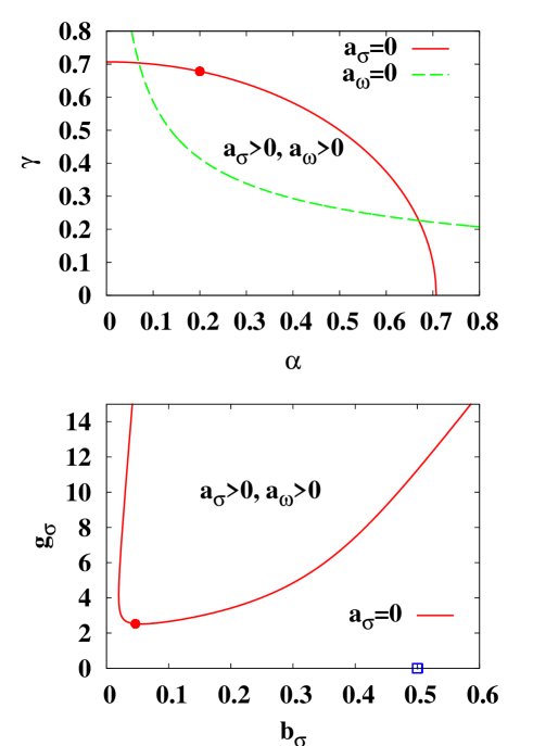
Figure 1: (Color online) Parameter range which satisfies the conditions of stability and high $T$ chiral symmetry restoration. The solid dot represents the parameter set, $\alpha=0.2,\alpha^{2}+\gamma^{2}=1/2-0$, which we adopt in the later discussion, and the square shows the parameter set without baryon effects.

By using the equilibrium condition, two auxiliary fields are related to each other, then we can obtain the effective free energy as a function of one order parameter. At equilibrium, the effective free energy is stationary with respect to $\sigma$ and $\omega$,

$${\partial{\cal F}_{{\rm eff}}\over\partial\sigma} = a_{\sigma}\sigma+a_{\sigma}{\partial F_{{\rm eff}}^{(q)}\over\partial{m_{q}}}=0\ ,$$ (59)

$${\partial{\cal F}_{{\rm eff}}\over\partial\omega} = a_{\omega}\omega+\alpha{\partial F_{{\rm eff}}^{(q)}\over\partial{m_{q}}}+{\partial\Delta F_{{\rm eff}}^{(b)}\over\partial\omega}=0\ .$$ (60)

The effects of $\Delta F_{{\rm eff}}^{(b)}$ is small when the fields are small, then in this case $\omega$ can be represented by the chiral condensate $\sigma$ as,

$${a_{\omega}\over\alpha}\omega\simeq\sigma=-{\partial F_{{\rm eff}}^{(q)}\over\partial{m_{q}}}=-{\partial{\cal F}_{{\rm eff}}\over\partial m_{0}}\ .$$ (61)

With this approximation for $\omega$, the effective free energy is given as a function of $\sigma$ as,

$${\cal F}_{{\rm eff}} = \frac{b_{\sigma}}{2}\sigma^{2}+F_{{\rm eff}}^{(q)}({m_{q}})+\Delta F_{{\rm eff}}^{(b)}(g_{\sigma}\sigma)\ ,$$ (62)

$${m_{q}} = b_{\sigma}\sigma+m_{0}\ ,$$ (63)

$$b_{\sigma} = a_{\sigma}+{\alpha^{2}\over a_{\omega}}\ ,\quad g_{\sigma}={\alpha g_{\omega}\over a_{\omega}}\ .$$ (64)

With this form of the effective free energy, the meaning of parameters are a little more clear. The constituent quark mass is a linear function of $\sigma$, then the coefficient $b_{\sigma}$ represents the polarizability of the chiral condensate, which is modified by the baryonic composite effects. The parameter $g_{\sigma}$ determines the strength of the coupling of the chiral condensate and the baryon, and $\Delta F_{{\rm eff}}^{(b)}(g_{\sigma}\sigma)$ represents the repulsive self-interaction of $\sigma$ coming from the baryon integral.

The parameters $b_{\sigma}$ and $g_{\sigma}$ are related to $\alpha$ and $\gamma$, and they have the region which satisfies the conditions of stability and high $T$ chiral symmetry restoration as shown in the lower panel of Fig. 1. We notice $\Delta F_{{\rm eff}}^{(b)}(g_{\sigma}\sigma)$ has the positive value for any $\sigma$, hence, the smaller $g_{\sigma}$ leads to smaller $\mathcal{F}_{\mathrm{eff}}$. Thus, we choose those parameters to give a small coupling $g_{\sigma}$ for a given polarizability $b_{\sigma}$. The smallest $g_{\sigma}$ at a fixed $b_{\sigma}$ is obtained in the limit of $a_{\sigma}\to+0$, or $\gamma^{2}+\alpha^{2}\to 1/2-0$. There is no singular behavior in the effective free energy in this limit as a function of the chiral condensate $\sigma$ in Eq. (62). For numerical calculations, we adopt $\alpha=0.2$, which gives almost the smallest $g_{\sigma}$ as shown by the filled circle in Fig. 1, as a typical value in the later discussion.

III Phase Structure

In the previous section, we have demonstrated that the effective action in the strong coupling limit lattice QCD can be obtained in an almost analytic way with $1/d$ expansion and mean field ansatz, when the diquark condensate is zero. Especially, we focus our attention to the chiral phase transition.

In this section, we discuss the phase diagram based on the effective free energy as a function of the chiral condensate in Eq. (62) in the chiral limit, $m_{0}=0$. Since we utilize the linear approximation ($a_{\omega}\omega/\alpha\simeq\sigma$, see Eq. (61)), equilibrium value of $\sigma$ slightly differs from that of $-\partial{\cal F}_{{\rm eff}}/\partial m_{0}=-\langle\bar{\chi}\chi\rangle$. However the difference of those is small and only by around 1 % as discussed in Subsec. III.3. For numerical calculations, we adopt a parameter choice of $\alpha=0.2$ and $\alpha^{2}+\gamma^{2}\to 1/2$, which gives $b_{\sigma}\simeq 0.0465$ and $g_{\sigma}\simeq 2.527$. This value of $g_{\sigma}$ is almost the smallest value allowed in this model.

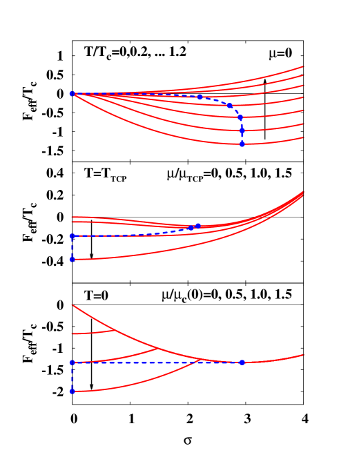
Figure 2: (Color online) Effective potential as a function of $\sigma$. Upper, middle, and lower panels show the effective free energies ${\cal F}_{{\rm eff}}$ in the unit of $T_{c}$ at $\mu=0$, $T=T_{\mathrm{TCP}}$, and $T=0$, respectively. Dots represent the equilibrium points, and dashed lines connect these points.

III.1 Zero temperature

It would be instructive to analyze several limits of the effective free energy Eq. (62). The effective free energy from the quark integral $F_{{\rm eff}}^{(q)}$ depends on the temperature and chemical potential. At zero temperature, $F_{{\rm eff}}^{(q)}$ can be reduced to

$$F_{{\rm eff}}^{(q)}({m_{q}};T\to 0,\mu)=\begin{cases}-N_{c}\,{E_{q}}&({E_{q}}>\mu)\ ,\\ -N_{c}\,\mu&({E_{q}}<\mu)\ ,\\ \end{cases}$$ (65)

where ${E_{q}}=\mathrm{arcsinh}\,m_{q}$ is a quark excitation energy. In vacuum in the chiral limit, $(T,\mu,m_{0})=(0,0,0)$, $F_{{\rm eff}}^{(q)}$ has a linear term in $\sigma$, while other parts of the effective free energy start with $\sigma^{2}$, then we necessarily have a finite equilibrium value of $\sigma$. On the other hand, for a finite chemical potential, $F_{{\rm eff}}^{(q)}$ becomes independent from $\sigma$ for small $\sigma$, and the effective free energy start with the quadratic term, $b_{\sigma}\sigma^{2}$ in the chiral limit. Then we have a local minimum at $\sigma=0$ when $\mu$ is finite even if it is very small, as shown in the bottom panel of Fig. 2. As a result, the first order chiral phase transition occurs at the chemical potential which satisfies,

$$-3\mu_{c}^{\mathrm{(1st)}}(T=0)={\cal F}_{{\rm eff}}(\sigma_{0};T=0,\mu=0)\ ,$$ (66)

where $\sigma_{0}$ stands for the vacuum equilibrium value of $\sigma$.

III.2 Small chemical potentials

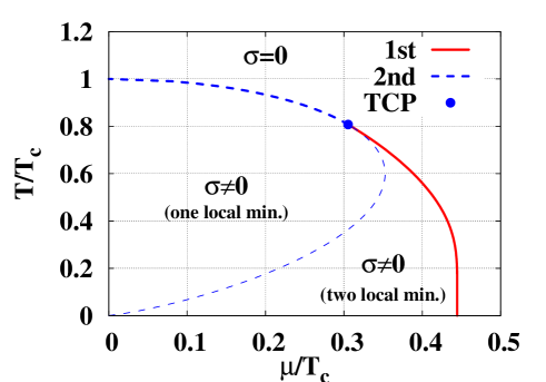
Figure 3: (Color online) Phase structure in the strong coupling limit lattice QCD with $N_{c}=3$. The solid (red) and upper thick dashed (blue) lines show the first and second order phase boundary, respectively. The dashed (blue) line shows the boundary on which the effective free energy curvature becomes zero at $\sigma=0$. The dot represents the tri-critical point (TCP). Chemical potential and temperature are shown in the unit of $T_{c}$.

At finite temperatures, we can expand $F_{{\rm eff}}^{(q)}$ in $\sigma^{2}$,

$$F_{{\rm eff}}^{(q)}(b_{\sigma}\sigma;T>0,\mu)$$ (67)

$$= -T\log\left({C_{3\mu}+2\over 3}\right)-{5b_{\sigma}^{2}\sigma^{2}\over T(C_{3\mu}+2)}+\Delta F_{{\rm eff}}^{(q)}\ ,$$

where $\Delta F_{{\rm eff}}^{(q)}={\cal O}(\sigma^{4})$. In the chiral limit, the coefficient of $\sigma^{2}$ in ${\cal F}_{{\rm eff}}$,

$$c_{2}(T,\mu)=\frac{1}{2}b_{\sigma}-{5b_{\sigma}^{2}\over T(C_{3\mu}+2)}\ ,$$ (68)

controls the second order phase transition. At zero chemical potential, this coefficient changes sign at

$$T_{c}=T_{c}^{\mathrm{(2nd)}}(\mu=0)={10b_{\sigma}\over 3}\ .$$ (69)

For lower temperatures, $T<T_{c}$, the coefficient changes sign at a chemical potential

$$\mu_{c}^{\mathrm{(2nd)}}(T)={T\over 3}\mathrm{arccosh}\,\left({3T_{c}\over T}-2\right)\ .$$ (70)

For larger chemical potentials, $\mu>\mu_{c}^{\mathrm{(2nd)}}(T)$, the effective free energy has a local minimum at $\sigma=0$, as already mentioned in the case of $T=0$. The above critical chemical potential $\mu_{c}^{\mathrm{(2nd)}}$ is shown by the dashed line in Fig. 3.

In the present model, the chiral phase transition is second order at small chemical potentials in the chiral limit. The coefficient $c_{2}$ is a decreasing function of $T$ for a fixed $\mu$ for $\mu/T\lesssim 0.588$. In addition, the higher order terms are positive when the chemical potential is small,

$$\Delta F_{{\rm eff}}^{(b)}+\Delta F_{{\rm eff}}^{(q)}\simeq c_{4}\sigma^{4}+{\cal O}(\sigma^{6})\ ,$$ (71)

$${c_{4}\over b_{\sigma}^{4}}={3a_{0}^{(b)}\over 28}\left({g_{\sigma}\Lambda\over 4b_{\sigma}}\right)^{4}+{20T^{2}-41+150/(C_{3\mu}+2)\over 12T^{3}(C_{3\mu}+2)}\ .$$

As a result, we do not have any local minimum at finite values of $\sigma$ giving smaller effective free energy than $\sigma=0$. Therefore, the above $T_{c}$ is the actual chiral phase transition temperature, and then the chiral phase transition is second order at zero and small chemical potentials in the chiral limit. The behavior of the effective free energy at $\mu=0$ is shown in the upper panel of Fig. 2.

III.3 Phase diagram

In previous subsections, we have discussed the properties of the effective free energy at small $\sigma$ in the chiral limit. In order to discuss the whole phase diagram, we show the results of numerical calculations in the chiral limit ($m_{0}=0$) with a parameter value $\alpha=0.2$ in this subsection.

Since the chiral phase transition is second order for small chemical potentials and is first order for small temperatures, we have to have a tri-critical point (TCP) in the phase boundary. At TCP, the finite equilibrium chiral condensate $\sigma$, which gives the same effective free energy as that for $\sigma=0$, approaches to zero. In Fig. 2, we show the effective free energy as a function of $\sigma$ at zero chemical potential (upper panel), zero temperature (bottom panel) and at the TCP temperature. We can find clear characteristic behavior of the first order phase transition at zero temperature and the second order phase transition at zero chemical potential. At $T=T_{\mathrm{TCP}}$, we see a marginal trend.

In Fig. 3, we show the phase diagram. The dashed line shows the critical chemical potential at which the coefficient of the quadratic term, $\sigma^{2}$, becomes zero. Outside of this dashed line, we necessarily have a local minimum at $\sigma=0$. At low temperatures, we have another local minimum at a finite value of $\sigma$, giving a lower value of the effective potential than that of $\sigma=0$. As a result, we have three regions in the $(T,\mu)$ plane: The quark-gluon plasma (QGP) phase where the chiral symmetry is restored, the region of $\mu<\mu_{c}^{\mathrm{(2nd)}}(T)$ where we have one local minimum at a finite value of $\sigma$, and the region $\mu_{c}^{\mathrm{(2nd)}}(T)<\mu<\mu_{c}^{\mathrm{(1st)}}$ where we have two local minima.

It is interesting to find that, with the current choice of the parameter, $\mu_{c}^{\mathrm{(1st)}}(T)$ smoothly decreases as the temperature increases, and it joins with $\mu_{c}^{\mathrm{(2nd)}}$ at TCP. In the present model with one order parameter $\sigma$, the slope of $\mu_{c}^{\mathrm{(1st)}}(T)$ (i.e. $d\mu_{c}^{(1st)}/dT$ ) in Fig. 3 has to be the same as that of $\mu_{c}^{\mathrm{(2nd)}}(T)$ in the vicinity of TCP. The first order phase transition condition of equilibrium and balance with ${\cal F}_{{\rm eff}}(0)$ can be solved as $4c_{2}c_{6}=c_{4}^{2}$ for the effective free energy ${\cal F}_{{\rm eff}}(\sigma)=c_{0}+c_{2}\sigma^{2}+c_{4}\sigma^{4}+c_{6}\sigma^{6}$. In the vicinity of TCP $c_{2},c_{4}={\cal O}(\Delta T,\Delta\mu)$ are small, then the above condition requires $c_{2}={\cal O}((\Delta T,\Delta\mu)^{2})$ leading to very small $c_{2}$ which should be on the second order phase transition line, provided that $c_{6}$ is finite at around TCP. Therefore, negative slope $d\mu_{c}^{(1st)}/dT<0$ around TCP is a consequence of larger TCP temperature giving a negative slope of $\mu_{c}^{\mathrm{(2nd)}}$, $T_{\mathrm{TCP}}>T_{x}\simeq 0.599\,T_{c}$. The TCP temperature is a solution of a simultaneous equation of $c_{4}=0$ and $\mu=\mu^{\mathrm{(2nd)}}_{c}(T)$,

$${T_{\mathrm{TCP}}\over T_{c}}={41\over 25}\left[1+\sqrt{1+{164\over 625}T_{c}^{2}\left(5+9T_{c}c_{4}^{(b)}/b_{\sigma}^{4}\right)}\right]^{-1}\ ,$$ (73)

where $c_{4}^{(b)}$ stands for the first term of $c_{4}$ in Eq. (III.2). In the present parameterization, the condition $T_{\mathrm{TCP}}>T_{x}$ is satisfied in a wide range, $0.0864\leq\alpha\leq 0.563$. On the other hand, when we ignore the baryonic action, we get $c_{4}^{(b)}=0$, $T_{c}=5/3$ Nishida2004b , then $T_{\mathrm{TCP}}\simeq 0.52\,T_{c}<T_{x}$.

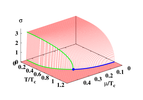
Figure 4: (Color online) Chiral condensate $\sigma$ as a function of chemical potential and temperature. Thick lines show the phase boundary, and the dot indicates the tri-critical point (TCP). Chemical potential and temperature are shown in the unit of $T_{c}$.

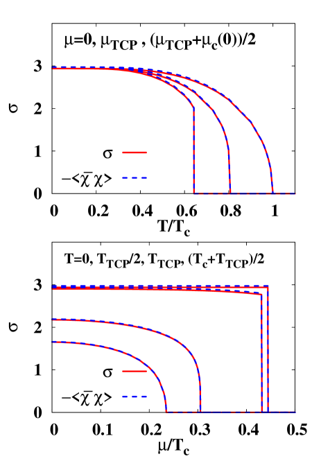
Figure 5: (Color online) Approximate chiral condensate $\sigma$ and the chiral condensate $-\partial{\cal F}_{{\rm eff}}/\partial m_{0}$ as a function of temperature (upper panel) and chemical potential (lower panel). Solid (red) and dashed (blue) lines show $\sigma$ and $-\langle\bar{\chi}\chi\rangle$, respectively. Chemical potential and temperature are shown in the unit of $T_{c}$.

In Figs. 5, we show the approximate chiral condensate $\sigma$ and the actual chiral condensate $\langle\bar{\chi}\chi\rangle=\partial{\cal F}_{{\rm eff}}/\partial m_{0}$ as a function of the temperature and chemical potential in the chiral limit. At zero temperature, the effective free energy is a common function of $\sigma$ in the region $\mathrm{arcsinh}\,\,b_{\sigma}\sigma>\mu$, and then the equilibrium value of $\sigma$ stays constant up to $\mu=\mu_{c}^{\mathrm{(1st)}}$. As a result, the equilibrium free energy is a constant when $\mu<\mu_{c}^{\mathrm{(1st)}}$, and decreases as ${\cal F}_{{\rm eff}}=\mathrm{const.}-N_{c}\mu$, leading to a sudden jump of the baryon density from $\rho_{\scriptscriptstyle B}=-\partial{\cal F}_{{\rm eff}}/\partial(N_{c}\mu)=0$ to $\rho_{\scriptscriptstyle B}=1$, which is the maximum value on the lattice. This behavior is an artifact of the strong coupling limit, and it is also found in previous works at zero temperature and finite chemical potential Bilic ; BilicCleymans ; Nishida2004b ; ZeroT:FiniteMu .

At finite temperatures, $\sigma$ smoothly decreases, and suddenly vanishes at $\mu_{c}^{\mathrm{(1st)}}$ when $T<T_{\mathrm{TCP}}$. The chiral condensate $\langle\bar{\chi}\chi\rangle$ is almost the same as $\sigma$. This approximate relation holds very well for small values of $\sigma$, and even for large values of $\sigma$ around the vacuum value, the ratio changes only by around 1 %.

IV Extended Examinations

The effective free energy derived and examined in the previous sections seems to be reasonable, and the calculated results qualitatively agree with those in other works. However, there are several unsatisfactory points. First, we have to introduce two parameters, $\gamma$ and $\alpha$. Several restrictions for these parameters are discussed in the previous section, and further discussions is presented in Subsec. IV.1. Secondly, we find quantitative differences in some thermodynamical variables from those in other works. In Subsec. IV.2, we compare the present effective free energy and other strong coupling limit models proposed so far. Thirdly, while we have shown that the diquark effect appears in several aspects of the effective free energy indirectly, it is unsatisfactory that we cannot treat the diquark condensate directly. In Subsec. IV.4, we propose an idea how to include the diquark condensate directly in the effective free energy.

IV.1 Parameter dependence

In the previous section, we have shown the relation between the scaled variables such as, $T/T_{c}$, $\mu/T_{c}$ and ${\cal F}_{{\rm eff}}/T_{c}$. This is because we can remove the major parameter dependence with these scaled variables at small $\sigma$ values. Here we would like to discuss that this scaling behavior corresponds to the modification of the lattice spacing.

When we explicitly put the spatial and temporal lattice spacings ($a$ and $a_{t}$) in the effective free energy, we find the following dependence.

$${\cal F}_{{\rm eff}} = {1\over a^{3}a_{t}}\left[\frac{1}{2}b_{\sigma}(a^{3}\sigma)^{2}+\Delta F_{{\rm eff}}^{(b)}(a^{3}g_{\sigma}\sigma)\right]$$ (74)

$$~{}~{}~{}~{}~{}-{T\over a^{3}}\log G_{U}(a_{t}a^{3}b_{\sigma}\sigma;a_{t}T,a_{t}\mu)\ ,$$

where $G_{U}=\exp(-F_{{\rm eff}}^{(q)}/T)=\int dU_{0}G(\mathbb{x})$. The critical temperature depends on both of $a_{t}$ and $a$ as $T_{c}=10a_{t}b_{\sigma}/3a^{2}$.

We require that the second order chiral restoration temperature should be described independently from parameter choice, when we choose the temporal and spatial lattice spacing appropriately. Actually, the effective free energy up to $\sigma^{2}$, which governs the second order chiral restoration at small $\mu$, is found to be independent from the parameter choice for a given $T_{c}$,

$${\cal F}_{{\rm eff}} = {T_{c}\over a^{3}}\left[{3\sigma_{a}^{2}\over 20}+\beta_{c}\Delta F_{{\rm eff}}^{(b)}\right.$$ (75)

$$~{}~{}\left.-{T\over T_{c}}\log G_{U}\left({3\sigma_{a}\over 10\beta_{c}};{T\over\beta_{c}T_{c}},{\mu\over\beta_{c}T_{c}}\right)\right]$$

$$= {T_{c}\over a^{3}}\left[{3\sigma_{a}^{2}\over 20}-{T\over T_{c}}\log G_{U}\right]+{\cal O}(\sigma^{3})\ ,$$

where $\sigma_{a}\equiv a^{4}\sigma/a_{t}$ stands for the chiral condensate measured in the unit of $a_{t}/a^{4}$ and $\beta_{c}=1/a_{t}T_{c}$ denotes the temporal lattice size at the critical temperature $T=T_{c}$. Since $\Delta F_{{\rm eff}}^{(b)}$ starts from $\sigma^{4}$ and $G_{U}$ is a function of $\mathrm{arcsinh}\,(b_{\sigma}\sigma)/T$ and $\mu/T$, the scaled effective free energy ${\cal F}_{{\rm eff}}/T_{c}$ is a function of scaled variables $\sigma_{a}$, $T/T_{c}$ and $\mu/T_{c}$ when we ignore ${\cal O}(\sigma^{3})$.

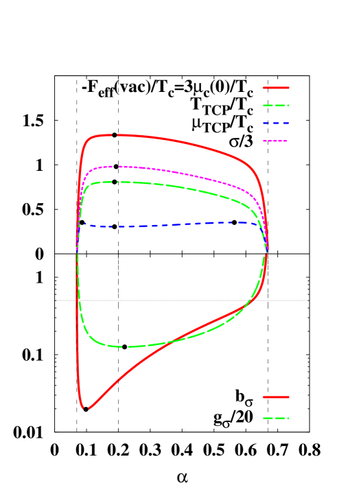
Figure 6: (Color online) Parameter dependence of $\mu_{c}(0)$ in vacuum (thick solid line, red), $T_{\mathrm{TCP}}$ (long dashed line, green), $\mu_{\mathrm{TCP}}$ (short dashed line, blue), and $\sigma$ (dotted line, magenta) in the upper graph. In the lower graph, thick solid line (red) and long dashed line (green) represents the parameter dependence of $b_{\sigma}$ and $g_{\sigma}$, respectively.

The remaining parameter dependence may come from the mean field ansatz. Thus the parameter should be chosen in the range where the mean field ansatz is valid; i.e. the dependence of obtained quantities is small. In Fig. 6, we show the parameter dependence of $\sigma$ in vacuum, $T_{\mathrm{TCP}}$, $\mu_{\mathrm{TCP}}$ and $\mu_{c}(0)$, which suffer from higher order contributions of $\sigma$. Most of these quantities have extrema at around $\alpha=0.2$ ($\alpha\simeq 0.188$ for $T_{\mathrm{TCP}}$, $\mu_{\mathrm{TCP}}$ and $mu_{c}(0)$, and $\alpha\simeq 0.193$ for $\sigma$ in vacuum). In addition, we find that the parameter dependence is not strong in the parameter range, $0.1\leq\alpha\leq 0.6$. It is worth to mention here that $b_{\sigma}$ is small enough at around $\alpha\simeq 0.2$ and it satisfies the even integer condition for $\beta_{c}=1/aT_{c}=3/10b_{\sigma}\geq 2$ in a symmetric lattice.

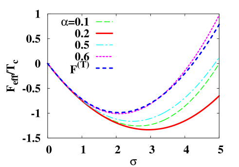
Figure 7: (Color online) Parameter dependence of the effective free energy in vacuum in the chiral limit, $(T,\mu,m_{0})=(0,0,0)$. Long dashed (green), thick solid (red), dash-dotted (light blue), and dotted (magenta) lines show the effective free energy in the present work, ${\cal F}_{{\rm eff}}^{(Tb)}$, with parameters $\alpha=$ 0.1, 0.2, 0.5 and 0.6, respectively. Short dashed line (blue) shows the effective free energy without baryon effects, ${\cal F}_{{\rm eff}}^{(T)}$.

In Figs. 7 and 8, we show the parameter dependence of the effective free energy in vacuum and the phase boundary. In these figures, we also plot the results with the effective free energy ${\cal F}_{{\rm eff}}^{(T)}$,

$${\cal F}_{{\rm eff}}^{(T)}=\frac{1}{2}b_{\sigma}^{(T)}\sigma^{2}+F_{{\rm eff}}^{(q)}({m_{q}})=T_{c}\left[{3\over 20}\sigma^{2}-{T\over T_{c}}\log G_{U}\right]\ ,\\$$ (76)

$${m_{q}}=b_{\sigma}^{(T)}\sigma+m_{0},\ b_{\sigma}^{(T)}={d\over 2N_{c}},\ T_{c}={10b_{\sigma}^{(T)}\over 3}=\frac{5}{3}\ ,$$ (77)

which is obtained by ignoring the baryon effects and integrating over $U_{0}$ exactly in a similar way to that in Ref. Bilic ; BilicCleymans ; Nishida2004b . It is clearly seen that large energy gain is obtained with $\alpha\simeq 0.2$, and the phase boundary extends to the larger $\mu$ direction. When we ignore baryon effects, the effective free energy and phase boundary with ${\cal F}_{{\rm eff}}^{(T)}$ roughly corresponds to those with $\alpha=0.6$ in the present model with baryons.

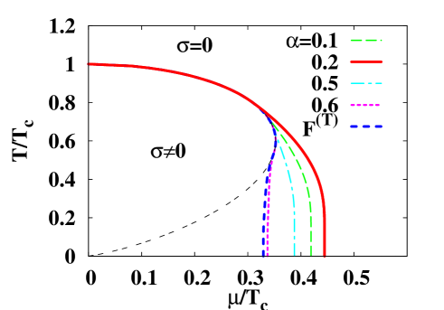
Figure 8: (Color online) Parameter dependence of the phase boundary. Long dashed (green), thick solid (red), dash-dotted (light-blue), and dotted (magenta) lines show the phase boundary in ${\cal F}_{{\rm eff}}$ with $\alpha=$0.1, 0.2, 0.5 and 0.6, respectively. Short dashed line (blue) shows the boundary in ${\cal F}_{{\rm eff}}^{(T)}$, without baryon effects. Thin solid line (black) indicates $c_{2}=0$, where $c_{2}$ is the quadratic coefficient of $\sigma$.

IV.2 Comparison with other treatments

While we have treated the time-like link variable $U_{0}$ exactly in the previous section, the anti-periodic boundary condition may not be very important when the temporary lattice size, $\beta=1/T$, is very large. In this case, it is possible to perform the one link integral also for $S_{F}^{(U_{0})}$ as other spatial action, $S_{F}^{(U_{j})}(j=1,2,3)$. After introducing auxiliary fields, $b,\bar{b}$ and $\sigma$, we obtain the action,

$$\int{\cal D}[U]e^{-S_{F}[U,\chi,\bar{\chi}]}\simeq\int{\cal D}[b,\bar{b},\sigma]e^{-S_{F}^{(0)}-S_{F}^{(m)}}\ ,$$ (78)

$$S_{F}^{(0)}[\chi,\bar{\chi},b,\bar{b},\sigma]=\frac{1}{2}\sum_{x,y}\sigma(x)V_{M0}(x,y)\sigma(y)$$

$$+\sum_{x,y}\left[\bar{b}(x)V_{B\mu}^{-1}(x,y)b(y)+\sigma(x)V_{M0}(x,y)M(y)\right]$$

$$-\sum_{x}\left[\bar{b}(x){B}(x)+\bar{B}(x)b(x)\right]\ ,$$ (79)

$$V_{M0}(x,y)={1\over 4N_{c}}\sum_{\nu=0}^{3}\left(\delta_{y,x+\hat{\nu}}+\delta_{y,x-\hat{\nu}}\right)\ ,$$ (80)

$$V_{B\mu}(x,y)=V_{B}-\frac{1}{8}\left(e^{3\mu}\delta_{y,x+\hat{0}}-e^{-3\mu}\delta_{y,x-\hat{0}}\right)\ .$$ (81)

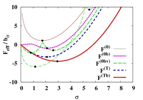
Figure 9: (Color online) Comparison of effective free energies in different treatments. Thin solid (red), dotted (magenta), long-dashed (green), and short-dashed (blue) lines show the effective free energies ${\cal F}_{{\rm eff}}^{(0)}$, ${\cal F}_{{\rm eff}}^{(0b)}$, ${\cal F}_{{\rm eff}}^{(0bv)}$ and ${\cal F}_{{\rm eff}}^{(T)}$, respectively. For ${\cal F}_{{\rm eff}}^{(0bv)}$ (long-dashed, green), we show the results with two parameters; $\alpha=\sqrt{1/2-\gamma^{2}}=0.2$ (thick) and $\gamma=2$ (thin). The thick solid line (red) indicates the effective free energy in a finite temperature treatment with baryon effects (${\cal F}_{{\rm eff}}^{(Tb)}$, present work). We show the results in vacuum in the chiral limit, $(T,\mu,m_{0})=(0,0,0)$.

In the above action, quark fields completely decouples in each space-time point, then it is possible to perform quark integral. For example, when we ignore the baryon effects and carry out the quark integral, we obtain the following effective free energy KS1981 ,

$${\cal F}_{{\rm eff}}^{(0)} = \frac{1}{2}b_{\sigma}^{(0)}\sigma^{2}-N_{c}\log(b_{\sigma}^{(0)}\sigma+m_{0})\ ,$$ (82)

where $b_{\sigma}^{(0)}=(d+1)/2N_{c}$ and ${m_{q}}=b_{\sigma}^{(0)}\sigma+m_{0}$. The diverging behavior at $\sigma=0$ in the chiral limit is suppressed when we include the baryon effects in a similar way to that in  DHK1985 ,

$${\cal F}_{{\rm eff}}^{\mathrm{(0b)}} = \frac{1}{2}b_{\sigma}^{(0)}\sigma^{2}+F_{{\rm eff}}^{(b\mu)}(4{m_{q}}^{3};T,\mu)\ .$$ (83)

The expression of the baryon integral, $F_{{\rm eff}}^{(b\mu)}$ is shown in the Appendix B. It is also possible to obtain the effective action with diquark field as,

$${\cal F}_{{\rm eff}}^{\mathrm{(0bv)}} = \frac{1}{2}b_{\sigma}^{(0)}\sigma^{2}+v^{2}-\log\Theta+F_{{\rm eff}}^{(b\mu)}(m;T,\mu)\ ,$$ (84)

$$\Theta = \frac{1}{3}\left(\frac{1}{R_{v}^{2}}-{{m_{q}}^{2}\over R_{v}\gamma^{2}}+\frac{2}{9}v^{2}\right)\ ,$$ (85)

$$m = {4{m_{q}}\left(3\gamma^{2}/R_{v}-{m_{q}}^{2}\right)\over\Theta}\ ,$$ (86)

where $R_{v}\equiv 1-v^{2}/3$. This effective free energy is essentially the same as that in Ref.  Azcoiti , while we use a different notation and introduce a parameter $\gamma$ as in the previous section.

These effective free energies have similar asymptotic behavior for large $\sigma$ in vacuum. Knowing the asymptotic form, $F_{{\rm eff}}^{(b\mu)}(m)\to-\log 2m$ at $m\to\infty$, we find all the potential terms in ${\cal F}_{{\rm eff}}^{(0)},{\cal F}_{{\rm eff}}^{(0b)}$ and ${\cal F}_{{\rm eff}}^{(0bv)}$, have the form of $-N_{c}\log\sigma+\mathrm{const.}$ in the large $\sigma$ limit. The effective free energy at finite $T$, ${\cal F}_{{\rm eff}}^{(T)}$ in Eq. (76), also has the potential of the above form, since $F_{{\rm eff}}^{(q)}(\sigma)\to-\log 2\sigma(\sigma\to\infty)$.

In Fig. 9, we compare the effective free energies as a function of the chiral condensate $\sigma$ in vacuum in the chiral limit. We show the scaled effective free energies ${\cal F}_{{\rm eff}}^{(i)}/b_{\sigma}^{(i)}$ instead of ${\cal F}_{{\rm eff}}^{(i)}/T_{c}$, since the chiral restoration does not emerge with zero temperature effective free energies, ${\cal F}_{{\rm eff}}^{(0)},{\cal F}_{{\rm eff}}^{(0b)},{\cal F}_{{\rm eff}}^{(0bv)}$. In ${\cal F}_{{\rm eff}}^{(0bv)}$, the diquark condensate $v$ is set to be zero, as the global minimum is already reported to lie at $v=0$ Azcoiti , and the results with two parameters are compared; the same parameter set as in the present work, $\gamma=\sqrt{1-\alpha^{2}}$ with $\alpha=0.2$, and the value originally adopted in Ref. Azcoiti , $\gamma=2$. From a comparison of ${\cal F}_{{\rm eff}}^{(0)}$ and ${\cal F}_{{\rm eff}}^{(0b)}$, the main role of baryons is found to reduce the effective free energy at small $\sigma$ values, in addition to suppressing the diverging behavior at $\sigma=0$. On the other hand, in zero temperature treatments with baryons, ${\cal F}_{{\rm eff}}^{(0b)}$ and ${\cal F}_{{\rm eff}}^{(0bv)}$, we find a bump at a small $\lambda$, which separates two local minima. This bump comes from the slow startup of the baryon contribution proportional to $\sigma^{6}$ at small $\sigma$ in ${\cal F}_{{\rm eff}}^{(0b)}$, and from a cancellation between $-\log\Theta$ and $F_{{\rm eff}}^{(b\mu)}(m)$ in ${\cal F}_{{\rm eff}}^{(0bv)}$. In a finite temperature treatment, ${\cal F}_{{\rm eff}}^{(T)}$, reduction effect is smooth, and we find only one local minimum. The effective free energy in the present work, ${\cal F}_{{\rm eff}}^{(Tb)}={\cal F}_{{\rm eff}}$ in Eq. (62), is smaller than those in other treatments except for ${\cal F}_{{\rm eff}}^{(0bv)}$ with $\gamma=2$, with which the effective free energy becomes unstable in a finite temperature treatment. The large energy gain in ${\cal F}_{{\rm eff}}^{(Tb)}$ may partly come from the scaling of ${\cal F}_{{\rm eff}}/b_{\sigma}$, since the $b_{\sigma}$ in this work is the smallest among the models compared here. In order to compare the absolute values of the effective free energy more seriously, it would be necessary to fix the lattice spacing and thus the energy scale and to include the effects of the higher order contribution in the $1/d$ expansion.

IV.3 Expected evolution of the phase diagram

One of the common problems in the strong coupling limit is the too small critical chemical potential $\mu_{c}(T=0)$ relative to $T_{c}=T_{c}(\mu=0)$. In Table 1, we compare the ratio of the critical baryon chemical potential at zero temperature with respect to the critical temperature at zero chemical potential, $R_{\mu T}\equiv 3\mu_{c}(T=0)/T_{c}$. All the models based on the strong coupling limit give much smaller values for this ratio, $R_{\mu T}<1.5$, than the empirical value, $R_{\mu T}=(1-2)\mathrm{GeV}/170\mathrm{MeV}\simeq(6-12)$. In the Monte-Carlo simulations at finite quark chemical potentials with finite $1/g^{2}$, it is not yet possible to obtain $\mu_{c}(T=0)$, but larger $R_{\mu T}$ values are suggested. For example, several Monte-Carlo methods are in agreement with each other for small quark chemical potentials $\mu/T<1$ LatticeFiniteMu ; Taylor ; AC ; Canonical ; FodorKatz , and the critical temperature for these chemical potentials are large enough, $T_{c}(\mu)/T_{c}(\mu=0)\gtrsim 0.9$, implying that $R_{\mu T}\gg 3$.

Table 1: Ratio of the critical chemical potential at zero temperature $\mu_{c}(T=0)$ and the critical temperature $T_{c}=T_{c}(\mu=0)$ in strong coupling models. In ${\cal F}_{{\rm eff}}^{(0b)}$, we have assumed $T_{c}=5/3$ to obtain the ratio. For the results in Ref. Bilic , values of critical lattice anisotropy $a/a_{t}$ and that multiplied by $\mu$ are taken for the number of staggered fermions, $f=1,2$ and 3.

Model	$T_{c}$	$\mu_{c}(T=0)$	$3\mu_{c}(0)/T_{c}$
${\cal F}_{{\rm eff}}^{(0b)}$ DHK1985		0.66	1.19	($T_{c}=5/3$)
${\cal F}_{{\rm eff}}^{(T)}$ Nishida2004b	$5/3$	0.33 $T_{c}$	0.99
${\cal F}_{{\rm eff}}^{(Tb)}$	$10b_{\sigma}/3$	0.45 $T_{c}$	1.34	($\alpha=0.2$)
Ref. Bilic	2.57	0.57	0.67	($f=1$)
	2.19	0.57	0.78	($f=2$)
	2.07	0.57	0.83	($f=3$)
Empirical	170 MeV	(1-2)/3 GeV	$\sim$ (6-12)

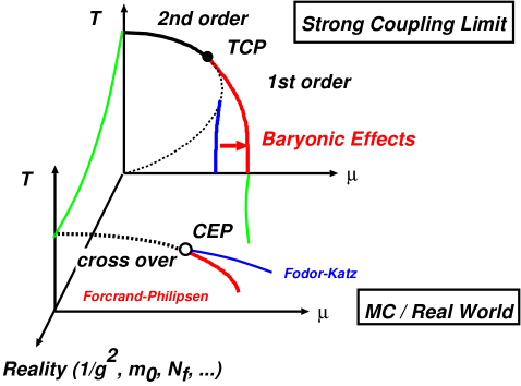
Figure 10: (Color online) Expected phase diagram evolution from the strong coupling limit in the chiral limit with one species of staggered fermion towards the real world.

Thus for a quantitative discussion, the strong coupling limit in the chiral limit with one species of staggered fermion is not enough, and it is necessary to take care of finite quark mass $m_{0}$, multi-staggered fermions, finite $1/g^{2}$, other order parameters than the chiral condensate, and/or other mechanisms towards the real world in order to explain large $\mu_{c}(T=0)$ relative to $T_{c}$, as illustrated in Fig. 10. With finite quark mass $m_{0}$, the effective free energy ${\cal F}_{{\rm eff}}$ always has a minimum at finite $\sigma$, then the second order boundary becomes cross over and the tri-critical point (TCP) becomes the critical end point (CEP). In addition, since the finite quark mass $m_{0}$ increases the baryon mass which is closely related to $\mu_{c}(T=0)$ DHK1985 , finite $m_{0}$ is believed to increase $\mu_{c}(T=0)$, as shown for example in Ref. Nishida2004b . With multi-staggered fermions, $T_{c}$ is suppressed as discussed in Ref. Bilic . It would be natural to expect that $T_{c}$ decreases as $1/g^{2}$ grows, because hadrons and glueballs are more bound at larger couplings and thus hadronic phase would be the most stable in the strong coupling limit. We further expect that the finite coupling effects appears most strongly at $\mu=0$, where the role of gluons relative to quarks is the largest. Actually in Ref. BilicCleymans , it is shown that $T_{c}(\mu)$ decreases as $1/g^{2}$ increases, and this reduction is more rapid at $\mu=0$ than at finite $\mu$.

With other order parameters than the chiral condensate, the phase diagram will have a richer structure. In Subsec. III.3, we have discussed that the slope of $\mu_{c}^{\mathrm{(1st)}}$ (see Fig. 3) have to be the same as that of $\mu_{c}^{\mathrm{(2nd)}}$ at the vicinity of TCP in the chiral limit with one order parameter. For this point, there is a debate between two Monte-Carlo simulations, one of which suggests the smooth connection of cross over boundary and the first order boundary Taylor ; AC ; Canonical , and the other suggests a finite difference in slope FodorKatz . Provided that the nature of TCP remains in CEP even with finite quark mass, our discussion in Subsec. III.3 supports the former if there is only one order parameter. However, both of the above two results can be consistent if there are other order parameters than the chiral condensate. Smooth connection is expected for chiral transition in methods based on the analyticity Taylor ; AC ; Canonical , while we may see other transition in a direct Monte-Carlo method at finite chemical potentials FodorKatz .

IV.4 Color angle average in diquark condensate

In deriving the effective free energy in Eq. (62) we have assumed that the diquark condensate takes zero values, $\phi_{a}=0$. If we ignore the diquark-gluon-baryon coupling, $S_{F}^{(C)}$ in Eq. (38), it is possible to obtain the solution of $\det\mathbb{g}_{ab}(k_{m})=0$ and the integral over $U_{0}$ numerically. With $S_{F}^{(C)}$, however, since $U_{0}$ depends on $\mathbb{x}$ and baryon fields are spatially connected through $\widetilde{V}_{B}$, we have to carry out the integral of baryon determinants over $2L^{3}$ dimensional variables in $U_{0}(\mathbb{x})$. In this subsection, we would like to show an idea to solve this problem in a case with one species of staggered fermion.

Since the diquark field $\phi_{a}$ is not color singlet, its average over the color space should be zero. Thus we cannot treat it as an order parameter. One of the way to remedy this problem is to carry out the integral of the ”color angle” variables in $\phi_{a}$, then only the color singlet combination $v^{2}=\phi_{a}^{\dagger}\phi_{a}$ remains. It is possible to carry out this color angle average in a straightforward way.

$$\Bigl{\langle}\exp\left[\sum_{a}\left(\phi_{a}^{\dagger}D_{a}+D_{a}^{\dagger}\phi_{a}\right)\right]\Bigr{\rangle}_{v}$$ (87)

$$= \Bigl{\langle}\prod_{a}\left[1+\phi_{a}^{\dagger}\phi_{a}D_{a}^{\dagger}D_{a}+\frac{1}{4}(\phi_{a}^{\dagger}\phi_{a})^{2}(D_{a}^{\dagger}D_{a})^{2}\right]\Bigr{\rangle}_{v}$$

$$= 1+\sum_{a}\langle\phi_{a}^{\dagger}\phi_{a}\rangle_{v}D_{a}^{\dagger}D_{a}+\frac{1}{4}\sum_{a}\langle(\phi_{a}^{\dagger}\phi_{a})^{2}\rangle_{v}(D_{a}^{\dagger}D_{a})^{2}$$

$$~{}~{}~{}+\sum_{a<b}\langle(\phi_{a}^{\dagger}\phi_{a})(\phi_{b}^{\dagger}\phi_{b})\rangle_{v}(D_{a}^{\dagger}D_{a})(D_{b}^{\dagger}D_{b})$$

$$= 1+{v^{2}\over 3}\sum_{a}D_{a}^{\dagger}D_{a}-{M^{3}\bar{b}{b}\over 54}\Bigl{\langle}\left(\sum_{a}\phi_{a}^{\dagger}\phi_{a}\right)^{2}\Bigr{\rangle}_{v}$$

$$= \exp\left({v^{2}\over 3}\sum_{a}D_{a}^{\dagger}D_{a}+{v^{4}\over 162}M^{3}\bar{b}{b}\right)\ .$$

Here we explicitly show the sum or product over color indices, and $\langle\cdots\rangle_{v}$ means the color angle average. When we integrate over the phase variable for each $\phi_{a}$, we only have those terms having the same power of $\phi_{a}$ and $\phi_{a}^{\dagger}$ as shown in the second line. The power of the diquark composite $D_{a}$ and $D^{\dagger}_{a}$ is limited to four as shown in the third line by the Grassmann nature. For example, the power four terms such as

$$\frac{1}{2}(D_{1}^{\dagger}D_{1})^{2}=(D_{1}^{\dagger}D_{1})(D_{2}^{\dagger}D_{2}) = -{1\over 27}M^{3}\bar{b}{b}\ ,$$ (88)

already contain all the Grassmann variables, and product with other $D_{a}$ or $D^{\dagger}_{a}$ vanishes. By using Eq. (88), we find that the fourth order terms in $D_{a}$ and $D_{a}^{\dagger}$ can be arranged in the form of $(\sum\phi_{a}^{\dagger}\phi_{a})^{2}=(v^{2})^{2}$. In the second order terms, we use the symmetry for each color index, for example, $\langle\phi_{1}^{\dagger}\phi_{1}\rangle_{v}=v^{2}/3$.

Unfortunately we again have the term containing the coupling of three-quark and baryon, $\bar{b}{B}+\bar{B}b$, from $D_{a}^{\dagger}D_{a}=Y+\bar{b}{B}+\bar{B}b$ (see Eq. (17)).

$$\exp(\bar{b}{B}+\bar{B}b)$$ (90)

$$= \int{\cal D}[v]e^{-v^{2}-Y}\Bigl{\langle}e^{\phi^{\dagger}D+D^{\dagger}\phi}\Bigr{\rangle}_{v}$$

$$= \int{\cal D}[v]e^{-v^{2}-Y+v^{2}\left(\bar{b}{B}+\bar{B}b+Y\right)/3+v^{4}M^{3}\bar{b}{b}/162}$$

$$\propto e^{v^{2}\left(\bar{b}{B}+\bar{B}b\right)/3-v^{2}-R_{v}Y+v^{4}M^{3}\bar{b}{b}/162}\ ,$$

$$R_{v}=1-v^{2}/3\ .$$

In the third line, we have assumed that the integral in r.h.s. can be approximated by the representative value of $v$. This approximation would be valid when the diquark condensate is strong. In this mean field ansatz, then we can solve this self-consistent relation as follows,

$$e^{R_{v}(\bar{b}{B}+\bar{B}b)} \simeq e^{-v^{2}-R_{v}Y+v^{4}M^{3}\bar{b}{b}/162}\ ,$$ (91)

where we have ignored the constant shift in the exponent. As a result, we obtain the following relation,

$$\exp(\bar{b}{B}+\bar{B}b) \simeq \exp\left[-{v^{2}\over R_{v}}+{v^{4}M^{3}\bar{b}{b}\over 162R_{v}}-Y\right]\ .$$ (92)

Coupling terms of $M^{n}\bar{b}{b}$ can be bosonized by introducing $n$ bosons, whose expectation values are related to the product of $\bar{q}q$ pair and $\bar{b}{b}$ pair $M^{k}\bar{b}{b}$, $\langle{\omega_{k}}\rangle=-\alpha_{k}\langle{M}\rangle+\beta_{k}\langle{M^{k}\bar{b}{b}}\rangle$, in a similar way to that in Sec. II. After introducing three auxiliary fields, $\omega_{2},\omega_{1},\omega_{0}$, it is possible to carry out the Grassmann variable integral, $b$ and $\chi$, and we obtain the effective free energy.

$${\cal F}_{{\rm eff}}^{(Tbv)} = F_{X}(\sigma,v,\omega_{i})+F_{{\rm eff}}^{(b)}(g_{\omega}\omega)+F_{{\rm eff}}^{(q)}({m_{q}})\ ,$$ (93)

$$F_{X} = \frac{1}{2}(a_{\sigma}\sigma^{2}+\omega^{2}+\omega_{1}^{2}+\omega_{2}^{2})+{v^{2}\over R_{v}}\ ,$$ (94)

$$a_{\sigma} = \frac{1}{2}-\gamma^{2}-\alpha^{2}-\alpha_{1}^{2}-\alpha_{2}^{2}\ ,$$ (95)

$${m_{q}} = a_{\sigma}\sigma+\alpha\omega+\alpha_{1}\omega_{1}+\alpha_{2}\omega_{2}+m_{0}\ ,$$ (96)

$$g_{\omega} = {1\over 9\alpha\gamma^{2}}\left[1+{\gamma^{2}v^{4}\omega_{1}\omega_{2}\over 18\alpha_{1}\alpha_{2}R_{v}}\right]\ .$$ (97)

Here we have replaced $\omega_{0}=\omega$ and $\alpha_{0}=\alpha$.

With zero diquark condensate, the effective free energy ${\cal F}_{{\rm eff}}^{(Tbv)}$ in Eq. (93), has a similar structure to ${\cal F}_{{\rm eff}}$ in Eq. (62). Specifically, when we take the linear approximation in the same way to that in Eq. (61), we find that the chiral condensate polarizability and the coupling constant are the same as before, $b_{\sigma}^{(Tbv)}=b_{\sigma},g_{\sigma}^{(Tbv)}=g_{\sigma}$ defined in Eq. (64), and we obtain the same effective free energy as before defined in Eq. (62),

$${\cal F}_{{\rm eff}}^{(Tbv)}(v=0)$$

$$\simeq\frac{1}{2}b_{\sigma}^{(Tbv)}\sigma^{2}+F_{{\rm eff}}^{(q)}(b_{\sigma}^{(Tbv)}\sigma+m_{0})+\Delta F_{{\rm eff}}^{(b)}(g_{\sigma}^{(Tbv)}\sigma)$$

$$~{}~{}={\cal F}_{{\rm eff}}\ .$$ (98)

This equivalence may serve a cross check of the effective free energy derived in Sec. II.

On the other hand, there is no potential effects proportional to $v^{2}$ while we have quadratic term in $F_{X}$, then we will not have any second order phase transition to the diquark condensed state. This comes from the cancellation in Eq. (92) in the case of one staggered fermion. Detailed analysis of the effective free energy Eq. (93) and its extension with multi-staggered fermions DKS1986 ; Bilic will be reported elsewhere.

V Summary

In this work, we have studied the phase diagram of QCD for color SU(3) at finite temperature ($T$) and finite chemical potential ($\mu$) by using an effective free energy derived in the strong coupling limit including baryon effects. We have adopted the effective action up to the next-to-leading order of the $1/d$ expansion (${\cal O}(1)$ and ${\cal O}(1/\sqrt{d})$), and by using the mean field ansatz, an analytical expression of the effective free energy is derived. The baryonic composite term in the effective action is decomposed into the terms consisting diquark condensates, baryons, and quarks Azcoiti . By introducing auxiliary fields of the baryon, diquark, baryon potential, and chiral condensate, we have obtained the effective action in the bilinear form of fermions. Then the Grassmann integral of quarks and the sum over the Matsubara frequency can be carried out exactly, provided that the solution of $\det\mathbb{g}_{ab}(k_{m})=0$ is obtained. At zero diquark condensate, we can further perform the integral over the temporal link variables and baryon fields analytically.

This is the first trial which introduces baryon and finite temperature effects simultaneously in the strong coupling limit of lattice QCD for color SU(3). It is important to note that baryon has effects to reduce the effective free energy ${\cal F}_{{\rm eff}}$ as shown in Fig. 7 and to extend the hadron phase to a larger $\mu$ direction at low temperatures as shown in Fig. 8, when ${\cal F}_{{\rm eff}}$, $\mu$ and $T$ are measured relative to $T_{c}$. We may expect that this feature remains in the realistic parameter region of finite $1/g^{2}$. It would then be interesting to compare the phase boundary behavior between SU(3) and U(3) to examine the baryon effects in this parameter region.

The obtained phase diagram have the second order phase boundary at small chemical potentials, and the first order phase boundary at small temperatures separated by a tri-critical point. This feature is the same as that in previous works, but the ratio of the critical baryon chemical potential at zero temperature with respect to the critical temperature at zero chemical potential, $R_{\mu T}\equiv 3\mu_{c}(T=0)/T_{c}(\mu=0)$, is found to be much smaller than the empirical value or that suggested in Monte-Carlo simulations. Small $R_{\mu T}$ is a common feature in models based on the strong coupling limit, and it would be necessary to extend in the direction of the reality axes in Fig. 10 for a quantitative discussions. On the other hand, we expect that Monte-Carlo simulations should reproduce the strong coupling results of the phase boundary including the small value of $R_{\mu T}$ at a large value of $g$.

Finally, we have proposed a method, color angle average in colored auxiliary fields, which enables us to extract a color singlet order parameter and to include the diquark condensate explicitly in the effective free energy.

One of the problems which we have found in this work is the parameter dependence of the effective free energy ${\cal F}_{{\rm eff}}$. During the bosonization, we have introduced two parameters, $\alpha$ and $\gamma$. Since these are introduced through identities, the results should not strongly depend on the parameter choice and in fact we have shown that we can absorb a major parameter dependence of ${\cal F}_{{\rm eff}}$ at small $\sigma$ values, which determines the second order chiral transition, in the choice of the lattice spacing. For the remaining parameter dependence, we have required that the scaled effective free energy ${\cal F}_{{\rm eff}}/T_{c}$ in vacuum becomes as small as possible, and we have adopted $\alpha=0.2$ and $\alpha^{2}+\gamma^{2}=1/2-0$. This choice of parameters results in the temporal lattice spacing of $\beta_{c}=1/aT_{c}(\mu=0)\simeq 6.45$ in a symmetric lattice. However, we have learned that $1/aT_{c}(\mu=0)$ is not large and less than two in the strong coupling Monte-Carlo simulations with one species of staggered fermion (without quarter root of the quark determinant as in the present work) ForcrandPrivate . It means that the parameter region, $0.5\leq\alpha\leq 0.6$, is preferred, rather than $\alpha\simeq 0.2$. Considering these situations, we have to agree that the baryonic effect on the phase diagram delicately depends on the choice of the parameter $\alpha$, and it is desired to find a general procedure to determine them.

There are several future issues to be studied further: The first one is an extensive analysis of the effective free energy at finite quark masses and/or with diquark condensates. Secondly, interesting and promising direction is to consider multi species of staggered fermions, since color superconductor is expected to emerge at high densities when multi quark flavors are introduced CSC .

Appendix A Sum over the Matsubara frequencies

The quark determinant $G(\mathbb{x})$ appeared in Eq. (43) is an even function of $k_{m}$, then it may be expressed as a polynomial of $\cos{k_{m}}$.

$$G(\mathbb{x}) \equiv \prod_{m=1}^{\beta/2}\mbox{det}\left[\mathbb{g}_{ab}(k_{m})\right]=\prod_{m=1}^{\beta}\mbox{det}\left[\mathbb{g}_{ab}(k_{m})\right]^{1/2}$$

$$= \prod_{m=1}^{\beta}\prod_{j=1}^{6}\left(\cos{k_{m}}-rY_{j}(\mathbb{x})\right)^{1/2}$$

where $r=1$. The derivative by $r$ reads

$${d\log{G}(\mathbb{x})\over dr} = \frac{1}{2}\sum_{m,j}{-Y_{j}\over\cos{k_{m}}-rY_{j}}$$ (99)

$$= {1\over 2\Omega}\sum_{j}\left[\oint{dz\over 2\pi i}{-Y_{j}\over\cos{z}-rY_{j}}{-i\beta\over 1+e^{i\beta z}}\right.$$

$$~{}~{}~{}~{}\left.-\sum_{z_{j}^{r}}{-Y_{j}\over-\sin{z_{j}^{r}}}{-i\beta\over 1+e^{i\beta z_{j}^{r}}}\right]$$

$$= {i\beta\over 2\Omega}\sum_{j,z_{j}^{r}}{Y_{j}\over\sin{z_{j}^{r}}}{1\over 1+\exp(i\beta z_{j}^{r})}$$

$$= {-i\beta\over 2\Omega}\sum_{j,z_{j}^{r}}{dz_{j}^{r}\over dr}{1\over 1+\exp(i\beta z_{j}^{r})}$$

$$= {d\over dr}{1\over 2\Omega}\sum_{j,z_{j}^{r}}\log\left(1+\exp(-i\beta z_{j}^{r})\right)\ .$$

In the contour integral, we have contributions from $z=k_{m}$ poles as well as $z=z_{j}^{r}$, whose sum becomes zero. Here $z_{j}^{r}$ is the solution of $\cos{z}=rY_{j}$, and $\Omega$ stands for the degeneracy for $z_{j}^{r}(+2n\pi i)$. In the second line from the bottom in Eq. (99), we have used the relation,

$${d\cos{z_{j}^{r}}\over dr}=-\sin{z_{j}^{r}}{dz_{j}^{r}\over dr}=Y_{j}\ .$$ (100)

Now we obtain $\log{G}$ up to a factor.

$$\log{G}(\mathbb{x})={1\over 2}\sum_{j}\sum_{z_{j}}\log\left(1+\exp(-i\beta z_{j})\right)+\mbox{const.}\ .$$ (101)

The sum over $z_{j}$ is understood as we ignore the degeneracy $2n\pi i$, but we still have two solutions in a pairwise way, $\pm z_{j}$, since $z_{j}$ is the solution of $\cos{z}=Y_{j}$. We choose one of them as a principle value.

$$\log{G}(\mathbb{x}) = {1\over 2}\sum_{j}\log\left[(1+e^{-i\beta z_{j}})(1+e^{i\beta z_{j}})\right]+\mathrm{const.}$$ (102)

$$= \frac{1}{2}\sum_{j}\log(1+\cos\beta z_{j})+{\rm const.}\ .$$

We ignore the constant terms in $\log{G}(\mathbb{x})$, and we get $G(\mathbb{x})$ as follows.

$$G(\mathbb{x})=\left[\prod_{j}\left(1+\cos\beta z_{j}(\mathbb{x})\right)\right]^{1/2}\ .$$ (103)

Appendix B Baryon Integral

In this appendix, we show how to obtain the baryon determinant $\mathrm{Det}(1+\omega V_{B})$.

First, we make a Fourier transformation of baryon field,

$$b_{m}(\mathbb{x})={1\over\sqrt{L^{3}}}\sum_{\mathbb{k}}e^{i\mathbb{k}\cdot\mathbb{x}}b_{m\mathbb{k}}\ ,\quad\mathbb{k}={2\pi\over L}(k_{1},k_{2},k_{3})\ .$$ (104)

The staggered factor $\eta_{j}(x)$ in $V_{B}$ connects four different momenta,

$$\mathbb{k}^{(1)}=(k_{1},k_{2},k_{3}) \quad\mathbb{k}^{(2)}=(k_{1}+\pi,k_{2},k_{3})\ ,$$ ,

$$\mathbb{k}^{(3)}=(k_{1}+\pi,k_{2}+\pi,k_{3}) \quad\mathbb{k}^{(4)}=(k_{1},k_{2}+\pi,k_{3})\ ,$$ ,

and two different frequencies, $m$ and $m+\beta/2$. As a result, $V_{B}$ is found to be block diagonal.

$$\sum_{m,n,\mathbb{k},\mathbb{k}^{\prime}}\left(\bar{b}_{m\mathbb{k}},V_{B}b_{n\mathbb{k}^{\prime}}\right)$$

$$= \sum_{k_{1},k_{2}=1}^{L/2}\sum_{k_{3}}^{L}\sum_{m=1}^{\beta/2}\begin{pmatrix}\bar{\mathbb{b}}_{m}&\bar{\mathbb{b}}_{m}^{\prime}\\ \end{pmatrix}\begin{pmatrix}0&\mathbb{S}(\mathbb{k})\\ \mathbb{S}(\mathbb{k})&0\\ \end{pmatrix}\begin{pmatrix}\mathbb{b}_{m}\\ \mathbb{b}_{m}^{\prime}\\ \end{pmatrix}\ ,$$

where $\mathbb{b}_{m}$ represents the baryon field with four different momenta,

$$\mathbb{b}_{m} = \left(b_{m\mathbb{k}^{(1)}},\ b_{m\mathbb{k}^{(2)}},\ b_{m\mathbb{k}^{(3)}},\ b_{m\mathbb{k}^{(4)}}\right)\ ,$$

$$\mathbb{b}_{m}^{\prime} = \mathbb{b}_{m+\beta/2}\ .$$ (107)

The matrix $\mathbb{S}$ represents how these different momentum states are connected through $\eta_{j}$,

$$\mathbb{S}=-{i\over 4}\begin{pmatrix}\sin k_{1}&\sin k_{2}&\sin k_{3}&0\\ \sin k_{2}&-\sin k_{1}&0&\sin k_{3}\\ \sin k_{3}&0&-\sin k_{1}&-\sin k_{2}\\ 0&\sin k_{3}&-\sin k_{2}&\sin k_{1}\\ \end{pmatrix}$$ (108)

It is interesting to find that the square of $\mathbb{S}$ becomes a $c$-number,

$$\mathbb{S}\cdot\mathbb{S}=-\frac{1}{16}s^{2}\mathbb{1}\ ,\quad(s^{2}=\sum_{j=1}^{3}\sin^{2}k_{j})\ .$$ (109)

Now we can evaluate the baryon integral,

$$\exp(-\beta L^{3}F_{{\rm eff}}^{(b)}) \equiv {\rm Det}V_{B}\int{\cal D}[b,\bar{b}]\exp\left[-\left(\bar{b},\widetilde{V}_{B}^{-1}b\right)\right]$$ (110)

$$= {\rm Det}\left[1+\omega V_{B}\right]$$

$$= \prod_{k_{1}=1}^{L/2}\prod_{k_{2}=1}^{L/2}\prod_{k_{3}=1}^{L}\prod_{m=1}^{\beta/2}{\rm det}\Biggl{[}\begin{pmatrix}1&\omega\mathbb{S}\\ \omega\mathbb{S}&1\\ \end{pmatrix}\Biggr{]}$$

$$= \prod_{k_{1}=1}^{L/2}\prod_{k_{2}=1}^{L/2}\prod_{k_{3}=1}^{L}\prod_{m=1}^{\beta/2}\left(1+\omega^{2}s^{2}/16\right)^{4}$$

$$= \prod_{\mathbb{k}}\left(1+\omega^{2}s^{2}/16\right)^{\beta/2}\ .$$

For very large spatial lattice size $L$, we can replace the sum by the integral,

$$F_{{\rm eff}}^{(b)}(\omega)=-{1\over 2L^{3}}\sum_{\mathbb{k}}\log\left[1+{\omega^{2}s^{2}\over 16}\right]$$

$$=-\frac{1}{2\pi^{3}}\int_{-\pi/2}^{\pi/2}dk_{1}\int_{-\pi/2}^{\pi/2}dk_{2}\int_{-\pi/2}^{\pi/2}dk_{3}\log\left[1+{\omega^{2}s^{2}\over 16}\right]$$

$$\simeq-\frac{a^{(b)}_{0}}{2}\left({4\pi\over 3}\Lambda^{3}\right)^{-1}\int_{0}^{\Lambda}4\pi k^{2}dk\log\left[1+{\omega^{2}k^{2}\over 16}\right]$$

$$=-a^{(b)}_{0}f^{(b)}({\omega\Lambda\over 4})\ .$$ (111)

In the fourth line, we have made an approximation to replace the average in a box to that in a sphere. With this approximation, the effective free energy from baryon integral can be represented by a function, $f^{(b)}(x)$,

$$f^{(b)}(x)\equiv{3\over 2x^{3}}\int_{0}^{x}k^{2}dk\log(1+k^{2})$$ (112)

$$= \frac{1}{2}\log(1+x^{2})-{1\over x^{3}}\left[\arctan{x}-x+{x^{3}\over 3}\right]\ .$$

From numerical studies, following normalization factor and the cut off,

$$a^{(b)}_{0}=1.0055\ ,\quad\Lambda={\pi\over 2}\times 1.01502\ ,$$ (113)

are found to give a good global fit of $F_{{\rm eff}}^{(b)}$.

The baryon determinant $F_{{\rm eff}}^{(b\mu)}$ in Eqs. (83) and (84) can be also evaluated by using a similar technique shown here. We show only the results here.

$$F_{{\rm eff}}^{(b\mu)}(m;T,\mu)$$

$$\equiv-{T\over L^{3}}\log\mathrm{Det}\left(m/4+V_{B\mu}\right)$$

$$=-{T\over 2L^{3}}\sum_{k_{0},\mathbb{k}}\log\left[m^{2}+\sin^{2}(k_{0}-3i\mu)+s^{2}\right]$$

$$=-{T\over L^{3}}\sum_{\mathbb{k}}\log\left[\cosh(\beta\mathrm{arcsinh}\,\sqrt{s^{2}+m^{2}})+C_{3\mu}\right]\ ,$$

where, $s^{2}=\sum_{j=1}^{3}\sin^{2}k_{j}$. In the numerical calculations in Subsec. IV.2, we have adopted the following approximation assuming that the spatial lattice size $L$ is large enough and that the average in a cubic box can be well approximated by the average in a sphere,

$$F_{{\rm eff}}^{(b\mu)}(m;T,\mu)$$

$$\simeq-a_{0}^{(b\mu)}T{3\over 4\pi\Lambda^{3}}\int^{\Lambda}d\mathbb{k}\log\left[C_{b}(\mathbb{k},m)+C_{3\mu}\right]\ ,$$ (115)

$$C_{b}(\mathbb{k},m)=\cosh\left[\beta\mathrm{arcsinh}\,\sqrt{\mathbb{k}^{2}+m^{2}}\right]\ ,$$ (116)

where the simple ansatz $a_{0}^{(b\mu)}=1$ and $\Lambda=\pi/2$ are used in the numerical calculations shown in Subsec IV.2.

References

- (1) For recent progresses, see, for example, Proc. of the 17th Int. Conf. on Ultra-Relativistic Nucleus-Nucleus Collisions (Quark Matter 2004), (Oakland, California, USA, 11-17 Jan. 2004), J. Phys. G 30, S633 (2004).
- (2) See, for example, F. Karsch, Lect. Notes Phys. 583, 209 (2002) [arXiv:hep-lat/0106019].
- (3) For recent discussions, see, for example, O. Philipsen, Proc. of the XXIII Int. Symp. on Lattice Field Theory, July 25-30, 2005, Dublin, Ireland, Proceedings of Science (http://pos.sissa.it/), to appear.
- (4) S. Tsuruta and A. G. W. Cameron, Can. J. Phys. 44, 1895 (1966); N. Itoh, Prog. Theor. Phys. 44 (1970) 291; V. R. Pandharipande Nucl. Phys. A 178, 123 (1971); N. K. Glendenning, Phys. Lett. B 114, 392 (1982); Nucl. Phys. A 493, 521 (1989); F. Weber and M. K. Weigel, Nucl. Phys. A 505, 779 (1989); Y. Sugahara and H. Toki, Prog. Theor. Phys. 92, 803 (1994); J. Schaffner and I. N. Mishustin, Phys. Rev. C 53, 1416 (1996); S. Balberg and A. Gal, Nucl. Phys. A 265, 435 (1997); M. Baldo, G. F. Burgio and H.-J. Schulze, Phys. Rev. C 58, 3688 (1998); I. Vidaña, A. Polls, A. Ramos, L. Engvik and M. Hjorth-Jensen, Phys. Rev. C 62, 035801 (2000); S. Nishizaki, T. Takatsuka and Y. Yamamoto, Prog. Theor. Phys. 108 (2002) 703; T. Takatsuka, S. Nishizaki, Y. Yamamoto and R. Tamagaki, Prog. Theor. Phys. 105 (2001) 179.
- (5) T. Kunihiro, T. Muto, T. Takatsuka, R. Tamagaki and T. Tatsumi, Prog. Theor. Phys. Suppl. 112, 1 (1993), and references therein.
- (6) A.B. Migdal, Nucl. Phys. A210, 421 (1972); R.F. Sawyer and D.J. Scalapino, Phys. Rev. D 7, 953 (1973).
- (7) D.B. Kaplan and A.E. Nelson, Phys. Lett. B 175, 57 (1986); G. E. Brown, C. H. Lee, M. Rho and V. Thorsson, Nucl. Phys. A 567, 937 (1994) [arXiv:hep-ph/9304204]. H. Fujii, T. Maruyama, T. Muto and T. Tatsumi, Nucl. Phys. A 597 (1996) 645. C.H. Lee, Phys. Rep. 275, 255 (1996), and references therein.
- (8) A. Iwazaki and O. Morimatsu, Phys. Lett. B 571, 61 (2003) [arXiv:nucl-th/0304005].
- (9) D. Bailin and A. Love, Phys. Rept. 107, 325 (1984); R. Rapp, T. Schafer, E. V. Shuryak and M. Velkovsky, Phys. Rev. Lett. 81, 53 (1998) [arXiv:hep-ph/9711396]; M. G. Alford, K. Rajagopal and F. Wilczek, Phys. Lett. B 422, 247 (1998) [arXiv:hep-ph/9711395]; M. G. Alford, Ann. Rev. Nucl. Part. Sci. 51, 131 (2001) [arXiv:hep-ph/0102047]; D. T. Son, Phys. Rev. D 59, 094019 (1999) [arXiv:hep-ph/9812287]; M. G. Alford, K. Rajagopal and F. Wilczek, Nucl. Phys. B 537, 443 (1999) [arXiv:hep-ph/9804403]; J. Berges and K. Rajagopal, Nucl. Phys. B 538, 215 (1999) [arXiv:hep-ph/9804233]; K. Iida and G. Baym, Phys. Rev. D 63, 074018 (2001) [Erratum-ibid. D 66, 059903 (2002)] [arXiv:hep-ph/0011229]; M. Iwasaki and T. Iwado, Phys. Lett. B 350, 163 (1995).
- (10) N. K. Glendenning, S. Pei and F. Weber, Phys. Rev. Lett. 79, 1603 (1997) [arXiv:astro-ph/9705235]; I. Bombaci, I. Parenti and I. Vidana, Astrophys. J. 614, 314 (2004) [arXiv:astro-ph/0402404].
- (11) A. K. Holme, E. F. Staubo, L. P. Csernai, E. Osnes and D. Strottman, Phys. Rev. D 40 (1989) 3735; D. H. Rischke, M. I. Gorenstein, H. Stoecker and W. Greiner, Phys. Lett. B 237, 153 (1990); T. Ishii and S. Muroya, Phys. Rev. D 46, 5156 (1992).
- (12) S. Muroya, A. Nakamura, C. Nonaka and T. Takaishi, Prog. Theor. Phys. 110, 615 (2003) [arXiv:hep-lat/0306031].
- (13) See, for example, K. Redlich, F. Karsch and A. Tawfik, J. Phys. G 30, S1271 (2004) [arXiv:nucl-th/0404009]; F. Karsch, Prog. Theor. Phys. Suppl. 153, 106 (2004) [arXiv:hep-lat/0401031], and references therein.
- (14) C.R. Allton, M. Doring, S. Ejiri, S.J. Hands, O. Kaczmarek, F. Karsch, E. Laermann, K. Redlich, Phys. Rev. D 71, 054508 (2005) [arXiv:hep-lat/0501030].
- (15) P. de Forcrand and O. Philipsen, Nucl. Phys. B642, 290 (2002); B673, 170 (2003); M. D’Elia and M. P. Lombardo, Phys. Rev. D 67, 014505 (2003) [arXiv:hep-lat/0209146].
- (16) S. Kratochvila and P. de Forcrand, PoS LAT2005, 167 (2005) [arXiv:hep-lat/0509143].
- (17) Z. Fodor and S. D. Katz, J. High Energy Phys. 03, 014 (2002) [arXiv:hep-lat/0106002].
- (18) P. Hasenfratz and F. Karsch, Phys. Lett. B 125, 308 (1983).
- (19) I. Barbour, N. E. Behilil, E. Dagotto, F. Karsch, A. Moreo, M. Stone and H. W. Wyld, Nucl. Phys. B 275, 296 (1986).
- (20) See, for example, T. Hatsuda and T. Kunihiro, Phys. Rept. 247, 221 (1994) [arXiv:hep-ph/9401310], and references therein.
- (21) K. Fukushima, Prog. Theor. Phys. Suppl. 153, 204 (2004) [arXiv:hep-ph/0312057].
- (22) E. Dagotto, F. Karsch and A. Moreo, Phys. Lett. B 169, 421 (1986); J. U. Klatke and K. H. Mutter, Nucl. Phys. B 342, 764 (1990).
- (23) Y. Nishida, K. Fukushima and T. Hatsuda, Phys. Rept. 398, 281 (2004) [arXiv:hep-ph/0306066].
- (24) N. Kawamoto, Nucl. Phys. B 190, 617 (1981).
- (25) N. Kawamoto and J. Smit, Nucl. Phys. B 192, 100 (1981).
- (26) J. Hoek, N. Kawamoto and J. Smit, Nucl. Phys. B 199, 495 (1982).
- (27) H. Kluberg-Stern, A. Morel and B. Petersson, Nucl. Phys. B 215, 527 (1983).
- (28) P. H. Damgaard, N. Kawamoto and K. Shigemoto, Phys. Rev. Lett. 53, 2211 (1984).
- (29) P. H. Damgaard, N. Kawamoto and K. Shigemoto, Nucl. Phys. B 264, 1 (1986).
- (30) P. H. Damgaard, D. Hochberg and N. Kawamoto, Phys. Lett. B 158, 239 (1985).
- (31) E. M. Ilgenfritz and J. Kripfganz, Z. Phys. C 29, 79 (1985).
- (32) V. Azcoiti, G. Di Carlo, A. Galante and V. Laliena, J. High Energy Phys. 0309, 014 (2003) [arXiv:hep-lat/0307019].
- (33) G. Faldt and B. Petersson, Nucl. Phys. B 265, 197 (1986).
- (34) N. Bilic, K. Demeterfi and B. Petersson, Nucl. Phys. B 377, 651 (1992); N. Bilic, F. Karsch and K. Redlich, Phys. Rev. D 45, 3228 (1992);
- (35) N. Bilic and J. Cleymans, Phys. Lett. B 355, 266 (1995) [arXiv:hep-lat/9501019].
- (36) Y. Nishida, Phys. Rev. D 69, 094501 (2004) [arXiv:hep-ph/0312371].
- (37) X. Q. Luo, Phys. Rev. D 70, 091504(R) (2004) [arXiv:hep-lat/0405019].
- (38) F. Karsch and K. H. Mutter, Nucl. Phys. B 313, 541 (1989).
- (39) N. Kawamoto and K. Shigemoto, Phys. Lett. B 114, 42 (1982). Nucl. Phys. B 237, 128 (1984);
- (40) See, for example, J. Zinn-Justin, Quantum Field Theory and Critical Phenomena, (Claredon Press, Oxford, 1989), Chapter 1.
- (41) E. B. Gregory, S. H. Guo, H. Kroger and X. Q. Luo, Phys. Rev. D 62, 054508 (2000) [arXiv:hep-lat/9912054]; M. Chavel, Phys. Rev. D 56, 5596 (1997) [arXiv:hep-lat/9704010]; R. Aloisio, V. Azcoiti, G. Di Carlo, A. Galante and A. F. Grillo, Phys. Lett. B 453 (1999) 275 [arXiv:hep-lat/9811033].
- (42) M. Golterman, Y. Shamir and B. Svetitsky, arXiv:hep-lat/0602026.
- (43) P. de Forcrand, private communication.