Abstract

We apply twisted boundary conditions to lattice QCD simulations of three-point correlation functions in order to access spatial components of hadronic momenta different from the integer multiples of $2\pi/L$. We calculate the vector and scalar form factors relevant to the $K\to\pi$ semileptonic decay and consider all the possible ways of twisting one of the quark lines in the three-point functions. We show that the momentum shift produced by the twisted boundary conditions does not introduce any additional noise and easily allows to determine within a few percent statistical accuracy the form factors at quite small values of the four-momentum transfer, which are not accessible when periodic boundary conditions are considered. The use of twisted boundary conditions turns out to be crucial for a precise determination of the form factor at zero-momentum transfer, when a precise lattice point sufficiently close to zero-momentum transfer is not accessible with periodic boundary conditions.

1 Introduction

In lattice simulations of QCD the spatial components of the hadronic momenta $p_{j}$ ($j=1,2,3$) are quantized. The specific quantized values depend on the choice of the boundary conditions (BCs) applied to the quark fields. The most common choice is the use of periodic BCs in the spatial directions

$$\psi(x+\hat{e}_{j}L)=\psi(x)~{},$$ (1)

that leads to

$$p_{j}=n_{j}\frac{2\pi}{L}~{},$$ (2)

where the $n_{j}$’s are integer numbers. Thus the smallest non-vanishing value of $p_{j}$ is given by $2\pi/L$, which depends on the spatial size of the (cubic) lattice ($V=L^{3}$). For instance a current available lattice may have $L=32~{}a$, where $a$ is the lattice spacing, and $a^{-1}\simeq 2.5$ GeV leading to $2\pi/L\simeq 0.5$ GeV. Such a value may represent a strong limitation of the kinematical regions accessible for the investigation of momentum dependent quantities, like e.g. form factors.

In Ref. [1] it was proposed to use twisted BCs for the quark fields

$$\widetilde{\psi}(x+\hat{e}_{j}L)=e^{2\pi i\theta_{j}}~{}\widetilde{\psi}(x)$$ (3)

which allows to shift the quantized values of $p_{j}$ by an arbitrary amount equal to $\theta_{j}2\pi/L$, namely

$$\widetilde{p}_{j}=\theta_{j}\frac{2\pi}{L}+p_{j}=\theta_{j}\frac{2\pi}{L}+n_{j}\frac{2\pi}{L}~{}.$$ (4)

The twisted BCs (3) can be shown [1] to be equivalent to the introduction of a U(1) background gauge field coupled to the baryon number and applied to quark fields satisfying usual periodic BCs (the Aharonov-Bohm effect). Moreover in Ref. [2] the twisted BCs were firstly implemented in a lattice QCD simulation of two-point correlation functions of pseudoscalar mesons. The energy-momentum dispersion relation was checked showing that the momentum shift $2\pi\theta_{j}/L$ is a true physical one.

The aim of the present paper is to explore the use of distinct twisted BCs for different fermion species in the calculation of the momentum dependence of lattice three-point correlators. We want both to establish whether twisted BCs are able to provide in practice form factors at small values of the momentum transfer not accessible with periodic BCs, and to estimate the level of statistical precision that can be achieved. The latter is an important point because the introduction of twisted BCs leads to a non-negligible increase of the computational time due to the need of producing new inversions of the Dirac equation for each quark momentum. We anticipate that the answer to both questions is positive: the twisted BCs are able to provide form factors at small values of the momentum transfer with a precision comparable to the one attainable with periodic BCs.

In this work we consider the case of the vector and scalar form factors relevant to the $K\to\pi$ semileptonic transition, which have been recently investigated using periodic BCs by the quenched simulations of Ref. [3], as well as by the $n_{f}=2$ and $n_{f}=2+1$ dynamical flavor simulations of Refs. [4] and [5], respectively. There are two reasons for our choice.

First, the theoretical uncertainty in the determination of the vector form factor at zero-momentum transfer, $f(0)$, presently dominates the corresponding uncertainty in the extraction of the value of the Cabibbo angle from $K_{\ell 3}$ decays. As shown in Ref. [3], an important source of uncertainty for $f(0)$ comes from the precision in the determination of the form factor slopes at zero-momentum transfer. Thus an interesting issue is to check whether the access to new lattice points at small values of the momentum transfer can improve significantly the precision of the determination of $f(0)$.

Second, the approach of Ref. [3] is characterized by the use of a suitable double ratio of three-point correlators, which allows to access in a very precise way the scalar form factor $f_{0}(q^{2})$ at $\vec{q}=0$ corresponding to $q^{2}=q_{\rm max}^{2}=(M_{K}-M_{\pi})^{2}$. The precision level of the values of $f_{0}(q_{\rm max}^{2})$ is crucial to achieve the percent accuracy for $f(0)$. However, there are cases in which it is not possible to get a lattice point sufficiently close to $q^{2}=0$ using periodic BCs. An important example is represented by some of the form factors entering hyperon semileptonic decays, like the weak magnetism, the weak electricity, the induced scalar and pseudoscalar form factors [6]. Thus, we have carried out an analysis of our lattice data for the $K\to\pi$ transition, but excluding the very accurate value $f_{0}(q_{\rm max}^{2})$. We consider this analysis representative of the cases where a precise lattice point close to or at zero-momentum transfer is not accessible with periodic BCs.

We limit ourselves to quenched simulations where the generation of gauge configurations is clearly independent of the BCs applied to the quark fields. We expect that the ability of twisted BCs to provide form factors at small values of the momentum transfer do not depend on the use of the quenched approximation, and therefore we are confident that our findings hold as well also in case of partially quenched and full QCD simulations.

We obtain the $K\to\pi$ vector and scalar form factors for quite small values of the four-momentum transfer, which are not accessible when periodic BCs are considered, without introducing any significant additional noise and within a few percent statistical accuracy. For completeness we consider all the possible ways of twisting one of the quark lines in the three-point functions.

When the precise lattice point for $f_{0}(q^{2})$ at $q^{2}=q_{\rm max}^{2}$ is not included in the analysis, the use of twisted BCs is crucial to allow a determination of $f(0)$ at a few percent statistical level. On the contrary, when the very accurate value $f_{0}(q_{\rm max}^{2})$ is included in the analysis, the impact of twisted BCs on the determination of the $K\to\pi$ form factors and their slopes at zero momentum transfer turns out to be marginal, while we remind it is expensive for the computational time. This result is due to the fact that:   i) the precision of the lattice points obtained with twisted BCs is not comparable to the one that can be achieved through the double ratio method of Ref. [3] at the particular kinematical point $q^{2}=q_{\rm max}^{2}$, which in turn is quite close to $q^{2}=0$ in the simulation of Ref. [3];   ii) the use of twisted BCs does not lead to a sufficient improvement of the precision with respect to the nearest space-like points obtained with periodic BCs.

The plan of the paper is as follows. In the next Section we briefly discuss the implementation of the twisted BCs for the evaluation of all the propagators required in this work. In Section 3 we present the calculation of two- and three-point correlation functions having twisted quark lines. In Section 4 we show our results for the scalar and vector form factors of the $K\to\pi$ transition, while in Section 5 we investigate the impact of the twisted BCs on the determination of the slopes of the vector and scalar form factors at zero momentum transfer. Finally Section 6 is devoted to our conclusions.

2 Lattice quark propagators with twisted BCs

On the lattice, for a given flavor, the quark propagator $S(x,0)\equiv\langle\psi(x)~{}\overline{\psi}(0)\rangle$, where $\langle\dots\rangle$ indicates the average over gauge field configurations, satisfies the following equation

$$\sum_{y}D(x,y)~{}S(y,0)=\delta_{x,0}$$ (5)

where $D(x,y)$ is the Dirac operator whose explicit form depends on the choice of the lattice QCD action. In what follows we work with Clover fermions and therefore $D(x,y)$ is given explicitly by

$$D(x,y) = \delta_{x,y}\left(am_{0}+4r\right)-\frac{1}{2}\sum_{\mu}\left\{\delta_{x,y-a\hat{\mu}}~{}(r-\gamma_{\mu})~{}U_{\mu}^{\phantom{\dagger}}(x)\right.$$ (6)

$$+ \left.\delta_{x,y+a\hat{\mu}}~{}(r+\gamma_{\mu})~{}U_{\mu}^{\dagger}(y)\right\}-\frac{c_{SW}~{}r}{32}~{}\sum_{\mu,\nu}~{}P_{\mu\nu}(x)~{}\sigma_{\mu\nu}~{}\delta_{x,y}~{},$$

where $U_{\mu}(x)$ is the gauge link, $P_{\mu\nu}(x)$ is the (symmetric) plaquette in the ($\mu,\nu$) plane and we have omitted Dirac and color indices for simplicity.

When the quark field satisfies the twisted BCs (3), the corresponding quark propagator $\widetilde{S}(x,0)\equiv\langle\widetilde{\psi}(x)~{}\overline{\widetilde{\psi}}(0)\rangle$ still satisfies Eq. (5) with the same Dirac operator $D(x,y)$ but with different BCs. Following Refs. [1, 2] one can redefine the quark field as $\psi_{\vec{\theta}}(x)=e^{-2\pi i\vec{\theta}\cdot\vec{x}/L}\widetilde{\psi}(x)$ in order to work always with periodic BCs on the fields. In such a way the new quark propagator $S^{\vec{\theta}}(x,0)\equiv\langle\psi_{\vec{\theta}}(x)~{}\overline{\psi}_{\vec{\theta}}(0)\rangle$ satisfies the following equation

$$\sum_{y}D^{\vec{\theta}}(x,y)~{}S^{\vec{\theta}}(y,0)=\delta_{x,0}$$ (7)

with a modified Dirac operator $D^{\vec{\theta}}(x,y)$ but periodic BCs. The new Dirac operator is related to Eq. (6) by simply rephasing the gauge links

$$U_{\mu}(x)\to U_{\mu}^{\vec{\theta}}(x)\equiv e^{2\pi ia\theta_{\mu}/L}~{}U_{\mu}(x)$$ (8)

with the four-vector $\theta$ given by ($0,\vec{\theta}$). Note that the plaquette $P_{\mu\nu}(x)$ is left invariant by the rephasing of the gauge links. In terms of $S^{\vec{\theta}}(x,y)$, related to the quark fields $\psi(x)$ with periodic BCs, the quark propagator $\widetilde{S}(x,y)$, corresponding to the quark fields $\widetilde{\psi}(x)$ with twisted BCs, is simply given by

$$\widetilde{S}(x,y)=e^{2\pi i\vec{\theta}\cdot(\vec{x}-\vec{y})/L}~{}S^{\vec{\theta}}(x,y)~{}.$$ (9)

3 Two- and three-point correlation functions with twisted quark lines

We are interested in calculating the $K^{0}\to\pi^{-}$ form factors of the weak vector current $V_{\mu}=\bar{s}\gamma_{\mu}u$, which are defined through the relation

$$\langle\pi(p^{\prime})|V_{\mu}|K(p)\rangle=f_{+}(q^{2})(p+p^{\prime})_{\mu}+f_{-}(q^{2})(p-p^{\prime})_{\mu}~{},$$ (10)

where $q^{2}=(p-p^{\prime})^{2}$. As usual, we express $f_{-}(q^{2})$ in terms of the so-called scalar form factor

$$f_{0}(q^{2})=f_{+}(q^{2})+\frac{q^{2}}{M_{K}^{2}-M_{\pi}^{2}}f_{-}(q^{2})$$ (11)

with $f_{0}(0)=f_{+}(0)$.

From Eq. (10) the form factors can be expressed as linear combinations of hadronic matrix elements of time and spatial components of the weak vector current. The latter can be obtained on the lattice by calculating two- and three-point correlation functions

$$C_{\mu}^{K\pi}(t_{x},t_{y},\vec{p},\vec{p}^{\,\prime}) = \sum_{\vec{x},\vec{y}}\langle O_{\pi}(t_{y},\vec{y})~{}\widehat{V}_{\mu}(t_{x},\vec{x})~{}O_{K}^{\dagger}(0)\rangle\,e^{-i\vec{p}\cdot\vec{x}+i\vec{p}^{\,\prime}\cdot(\vec{x}-\vec{y})}\,\,,$$ (12)

$$C^{K(\pi)}(t,\vec{p}) = \sum_{\vec{x}}\langle O_{K(\pi)}(t,\vec{x})~{}O_{K(\pi)}^{\dagger}(0)\rangle\,e^{-i\vec{p}\cdot\vec{x}}\,\,,$$ (13)

where $O_{\pi}^{\dagger}=\bar{d}\gamma_{5}u$, $O_{K}^{\dagger}=\bar{d}\gamma_{5}s$ are the operators interpolating $\pi^{-}$ and $K^{0}$ mesons, and $\widehat{V}_{\mu}$ is the renormalized lattice vector current

$$\widehat{V}^{\mu}=Z_{V}\left(1+b_{V}\frac{am_{s}+am_{\ell}}{2}\right)\left(\bar{s}\gamma^{\mu}u+c_{V}\partial_{\nu}~{}\bar{s}\sigma^{\mu\nu}u\right)\,,$$ (14)

where $Z_{V}$ is the vector renormalization constant, $b_{V}$ and $c_{V}$ are $O(a)$-improvement coefficients and the subscript $\ell$ refers to the light $u$ (or $d$) quark. In what follows we always use degenerate $u$ and $d$ quarks.

Using the completeness relation and taking $t_{x}$ and $(t_{y}-t_{x})$ large enough, one gets

$$C_{\mu}^{K\pi}(t_{x},t_{y},\vec{p},\vec{p}^{\,\prime})~{}_{\overrightarrow{\stackrel{{\scriptstyle\mbox{\tiny$t_{x}\to\infty$}}}{{\mbox{\tiny$(t_{y}-t_{x})\to\infty$}}}}}~{}\frac{\sqrt{Z_{K}Z_{\pi}}}{4E_{K}E_{\pi}}\langle\pi(p^{\prime})|\widehat{V}_{\mu}|K(p)\rangle\,e^{-E_{K}t_{x}-E_{\pi}(t_{y}-t_{x})}\,,$$ (15)

$$C^{K(\pi)}(t,\vec{p}(\vec{p}^{\,\prime})) {}_{\overrightarrow{{\mbox{\tiny$t\to\infty$}}}} \frac{Z_{K(\pi)}}{2E_{K(\pi)}}e^{-E_{K(\pi)}t}\,,$$ (16)

where $E_{K}=\sqrt{M_{K}^{2}+|\vec{p}|^{2}}$, $E_{\pi}=\sqrt{M_{\pi}^{2}+|\vec{p}^{\,\prime}|^{2}}$ and $\sqrt{Z_{K(\pi)}}=\langle 0|O_{K(\pi)}(0)|K(\pi)\rangle$. Then it follows

$$\frac{C_{\mu}^{K\pi}(t_{x},t_{y},\vec{p},\vec{p}^{\,\prime})}{C^{K}(t_{x},\vec{p})~{}C^{\pi}(t_{y}-t_{x},\vec{p}^{\,\prime})}\left.{}_{\overrightarrow{\stackrel{{\scriptstyle\mbox{\tiny$t_{x}\to\infty$}}}{{\mbox{\tiny$(t_{y}-t_{x})\to\infty$}}}}}\right.\frac{\langle\pi(p^{\prime})|\widehat{V}_{\mu}|K(p)\rangle}{\sqrt{Z_{K}Z_{\pi}}}\,.$$ (17)

Consequently the hadronic matrix elements $\langle\pi(p^{\prime})|\widehat{V}_{\mu}|K(p)\rangle$ can be obtained from the plateaux of the l.h.s. of Eq. (17), once $Z_{K}$ and $Z_{\pi}$ are separately extracted from the large-time behavior of the two-point correlators (16).

In terms of the strange and light quark propagators $S_{s}(x,y)$ and $S_{\ell}(x,y)$ the two-point correlator $C^{K(\pi)}(t,\vec{p}(\vec{p}^{\,\prime}))$ becomes

$$C^{K(\pi)}(t,\vec{p}(\vec{p}^{\,\prime}))=\sum_{\vec{x}}\langle Tr[S_{\ell}(x,0)\gamma_{5}S_{s(\ell)}(0,x)\gamma_{5}]\rangle e^{-i\vec{p}(\vec{p}^{\,\prime})\cdot\vec{x}}$$ (18)

where $S_{s(\ell)}(0,x)=\gamma_{5}S_{s(\ell)}^{\dagger}(x,0)\gamma_{5}$. Analogously the three-point correlator $C_{\mu}^{K\pi}(t_{x},t_{y},\vec{p},\vec{p}^{\,\prime})$ becomes

$$C_{\mu}^{K\pi}(t_{x},t_{y},\vec{p},\vec{p}^{\,\prime})=\sum_{\vec{x}}\langle Tr[\Sigma_{\ell}(x,0;t_{y},\vec{p}^{\,\prime})\gamma_{\mu}S_{s}(0,x)]\rangle e^{-i\vec{q}\cdot\vec{x}}$$ (19)

where the generalized propagator $\Sigma(x,0;t_{y},\vec{p}^{\,\prime})$ satisfies the equation [9]

$$\sum_{z}D(x,z)~{}\Sigma(z,0;t_{y},\vec{p}^{\,\prime})=\gamma_{5}S(x,0)e^{-i\vec{p}^{\,\prime}\cdot\vec{x}}~{}\delta_{t_{x},t_{y}}~{}.$$ (20)

Using the twisted propagators, $\widetilde{S}$ and $\widetilde{\Sigma}$, Eqs. (18)-(20) hold as well taking into account the corresponding change of the quantized momenta ($p_{j}\to\widetilde{p}_{j}$). The new two- and three-point correlators can be always expressed in terms of quark propagators satisfying periodic BCs, namely Eq. (7). For the case of our interest and adopting in what follows the convention that the values of the momenta $\vec{p}$ and $\vec{p}^{\,\prime}$ are always given by multiples of $2\pi/L$, we get

$$C^{K^{0}}(t,\frac{2\pi}{L}(\vec{\theta}_{3}-\vec{\theta}_{1})+\vec{p}) = \sum_{\vec{x}}\langle Tr[S_{d}^{\vec{\theta}_{3}}(x,0)\gamma_{5}S_{s}^{\vec{\theta}_{1}}(0,x)\gamma_{5}]\rangle e^{-i\vec{p}\cdot\vec{x}}$$

$$C^{\pi^{-}}(t,\frac{2\pi}{L}(\vec{\theta}_{3}-\vec{\theta}_{2})+\vec{p}^{\,\prime}) = \sum_{\vec{x}}\langle Tr[S_{d}^{\vec{\theta}_{3}}(x,0)\gamma_{5}S_{u}^{\vec{\theta}_{2}}(0,x)\gamma_{5}]\rangle e^{-i\vec{p}^{\,\prime}\cdot\vec{x}}$$ (21)

$$C_{\mu}^{K^{0}\pi^{-}}(t_{x},t_{y},\frac{2\pi}{L}(\vec{\theta}_{3}-\vec{\theta}_{1})+\vec{p},\frac{2\pi}{L}(\vec{\theta}_{3}-\vec{\theta}_{2})+\vec{p}^{\,\prime})=\sum_{\vec{x}}e^{-i\vec{q}\cdot\vec{x}}$$

$$\langle Tr[\Sigma_{ud}^{\vec{\theta}_{2},\vec{\theta}_{3}}(x,0;t_{y},\vec{p}^{\,\prime})\gamma_{\mu}S_{s}^{\vec{\theta}_{1}}(0,x)]\rangle$$

$$C_{\mu}^{\pi^{-}K^{0}}(t_{x},t_{y},\frac{2\pi}{L}(\vec{\theta}_{3}-\vec{\theta}_{1})+\vec{p},\frac{2\pi}{L}(\vec{\theta}_{3}-\vec{\theta}_{2})+\vec{p}^{\,\prime})=\sum_{\vec{x}}e^{-i\vec{q}\cdot\vec{x}}$$

$$\langle Tr[\Sigma_{sd}^{\vec{\theta}_{2},\vec{\theta}_{3}}(x,0;t_{y},\vec{p}^{\,\prime})\gamma_{\mu}S_{u}^{\vec{\theta}_{1}}(0,x)]\rangle$$ (22)

where $\vec{q}=\vec{p}-\vec{p}^{\,\prime}$ and the generalized propagator $\Sigma_{q_{2}q_{3}}^{\vec{\theta}_{2},\vec{\theta}_{3}}$ is solution of the modified equation

$$\sum_{z}D_{q_{2}}^{\vec{\theta}_{2}}(x,z)~{}\Sigma_{q_{2}q_{3}}^{\vec{\theta}_{2},\vec{\theta}_{3}}(z,0;t_{y},\vec{p}^{\,\prime})=\gamma_{5}S_{q_{3}}^{\vec{\theta}_{3}}(x,0)e^{-i\vec{p}^{\,\prime}\cdot\vec{x}}~{}\delta_{t_{x},t_{y}}~{}.$$ (23)

To help visualizing the notation used for the $\theta$-vectors the three-point correlator relevant for the $K^{0}\to\pi^{-}$ semileptonic transition is depicted in Fig. 1 .

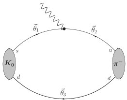
Fig. 1: Three-point correlation function of the $K^{0}\to\pi^{-}$ semileptonic transition with the various quark lines twisted by the vectors $\vec{\theta}_{1}$, $\vec{\theta}_{2}$ and $\vec{\theta}_{3}$.

Note that in the r.h.s. of Eqs. (21)-(23) the exponentials do not contain any $\theta$-vector because of Eq. (9).

4 Results for the $K\to\pi$ form factors

We have generated $100$ quenched gauge field configurations on a $24^{3}\times 56$ lattice at $\beta=6.20$ (corresponding to an inverse lattice spacing equal to $a^{-1}\simeq 2.6$ GeV), with the plaquette gauge action. Using non-perturbatively $O(a)$-improved Wilson fermions we have chosen quark masses corresponding to one pair of the values adopted in Ref. [3], namely $k\in\{0.1339,0.1349\}$.

Using $K$ and $\pi$ mesons with quark content ($k_{s}k_{\ell}$) and ($k_{\ell}k_{\ell}$) respectively, two different $K\to\pi$ correlators ($C_{\mu}^{K\pi}$) have been computed, using both $k_{s}<k_{\ell}$ and $k_{s}>k_{\ell}$, corresponding to the cases in which the kaon(pion) is heavier than the pion(kaon). Using the same combinations of quark masses, also the three-point $\pi\to K$ correlations ($C_{\mu}^{\pi K}$) have been calculated. Finally, two non-degenerate $K\to K$ and two degenerate $\pi\to\pi$ three-point functions have been evaluated.

As for the critical hopping parameter, we have adopted the value $k_{c}=0.135820(2)$ found in Ref. [3] using the axial Ward identity, and we have chosen the time insertion of the vector current equal to $t_{y}=T/2$, which allows to average the three-point correlators between the left and right halves of the lattice. Using the degenerate $K\to K$ and $\pi\to\pi$ transitions, for which the vector form factor at zero-momentum transfer is known to be equal to unity because of vector current conservation, the values of the renormalization constant $Z_{V}$ and of the $O(a)$-improvement parameter $b_{V}$, appearing in Eq. (14), are found to be in good agreement with the corresponding results of Ref. [3]. Finally, we adopt for the improvement coefficient $c_{V}$ the same non-perturbative value $c_{V}=-0.09$ used in Ref. [3]. Throughout this paper the statistical errors are evaluated using the jacknife procedure.

As shown in Ref. [3] the scalar form factor $f_{0}(q^{2})$ can be calculated very efficiently at $q^{2}=q_{\rm max}^{2}=(M_{K}-M_{\pi})^{2}$ using a double ratio of three-point correlation functions with both mesons at rest, namely

$$R_{0}(t_{x},t_{y})\equiv\frac{C_{0}^{K\pi}(t_{x},t_{y},\vec{0},\vec{0})\,C_{0}^{\pi K}(t_{x},t_{y},\vec{0},\vec{0})}{C_{0}^{KK}(t_{x},t_{y},\vec{0},\vec{0})\,C_{0}^{\pi\pi}(t_{x},t_{y},\vec{0},\vec{0})}~{}_{\overrightarrow{\stackrel{{\scriptstyle\mbox{\tiny$t_{x}\to\infty$}}}{{\mbox{\tiny$(t_{y}-t_{x})\to\infty$}}}}}~{}[f_{0}(q^{2}_{\rm max})]^{2}\,\frac{(M_{K}+M_{\pi})^{2}}{4M_{K}M_{\pi}}~{}.$$ (24)

For $q^{2}\neq q_{\rm max}^{2}$ the form factors $f_{+}(q^{2})$ and $f_{0}(q^{2})$ can be determined from the matrix elements of the time and spatial components of the vector current, $\langle\pi|\widehat{V}_{0}|K\rangle$ and $\langle\pi|\widehat{V}_{i}|K\rangle$ ($i=x,y,z$), that in turn can be extracted from the plateaux of the l.h.s. of Eq. (17) (as discussed in the previous Section). However, such a plain strategy leads to a determination of $f_{0}(q^{2})$ with a quite poor precision (see Ref. [3]). Therefore in order to achieve a much better accuracy we follow Ref. [3] and introduce a suitable ratio of the spatial and time components $\langle\pi|\widehat{V}_{0}|K\rangle$ and $\langle\pi|\widehat{V}_{i}|K\rangle$, normalized by the corresponding degenerate $K\to K$ transition, namely

$$R_{i0}\equiv\frac{\langle\pi|\widehat{V}_{i}|K\rangle}{\langle\pi|\widehat{V}_{0}|K\rangle}\frac{\langle K|\widehat{V}_{0}|K\rangle}{\langle K|\widehat{V}_{i}|K\rangle}~{},$$ (25)

which allows to access the ratio $f_{-}(q^{2})/f_{+}(q^{2})$.

First of all, as a consistency check of our run, we have evaluated the two- and three-point correlation functions (18) and (19) setting all the three $\theta$-vectors to zero and adopting the same values of $\vec{p}$ and $\vec{p}^{\,\prime}$ used in Ref. [3], where a different, larger set of $230$ quenched gauge configurations were employed. The results obtained for both $f_{0}(q_{\rm max}^{2})$ and the scalar and vector form factors at $q^{2}\neq q_{\rm max}^{2}$ are nicely consistent within the statistical errors. In what follows we will label these results as “$\theta=0$”. Then, the two- and three-point correlation functions (21) and (22) have been evaluated choosing always $\vec{p}=\vec{p}^{\,\prime}=0$ and making three different kinematical choices that correspond to assuming non-vanishing only one out of the three $\theta$-vectors of Fig. 1. Defining $Q\equiv 2\pi|\vec{\theta}|/L$, $E_{K}\equiv\sqrt{M_{K}^{2}+Q^{2}}$ and $E_{\pi}\equiv\sqrt{M_{\pi}^{2}+Q^{2}}$ we consider

• Kinematics A: $\vec{\theta}_{1}=\vec{\theta}\neq 0$ and $\vec{\theta}_{2}=\vec{\theta}_{3}=0$ ($\Rightarrow\vec{p}_{K}=2\pi\vec{\theta}/L$, $\vec{p}_{\pi}=\vec{0}$)

  $$f_{+}(q^{2}) = \frac{1}{2M_{\pi}}\left[\langle\pi|\widehat{V}_{0}|K\rangle-\frac{E_{K}-M_{\pi}}{Q}\langle\pi|\widehat{V}_{i}|K\rangle\right]$$

  $$f_{0}(q^{2}) = f_{+}(q^{2})\left[1+\frac{q^{2}}{M_{K}^{2}-M_{\pi}^{2}}\frac{(E_{K}+M_{\pi})R_{i0}-(M_{K}+E_{K})}{M_{K}+E_{K}-(E_{K}-M_{\pi})R_{i0}}\right]$$

  $$q^{2} = M_{K}^{2}+M_{\pi}^{2}-2M_{\pi}E_{K}=q_{\rm max}^{2}-2M_{\pi}(E_{K}-M_{K})~{};$$ (26)

• Kinematics B: $\vec{\theta}_{2}=\vec{\theta}\neq 0$ and $\vec{\theta}_{1}=\vec{\theta}_{3}=0$ ($\Rightarrow\vec{p}_{K}=\vec{0}$, $\vec{p}_{\pi}=2\pi\vec{\theta}/L$)

  $$f_{+}(q^{2}) = \frac{1}{2M_{K}}\left[\langle\pi|\widehat{V}_{0}|K\rangle-\frac{E_{\pi}-M_{K}}{Q}\langle\pi|\widehat{V}_{i}|K\rangle\right]$$

  $$f_{0}(q^{2}) = f_{+}(q^{2})\left[1+\frac{q^{2}}{M_{K}^{2}-M_{\pi}^{2}}\frac{M_{K}+E_{K}-(E_{\pi}+M_{K})R_{i0}}{M_{K}+E_{K}-(E_{\pi}-M_{K})R_{i0}}\right]$$

  $$q^{2} = M_{K}^{2}+M_{\pi}^{2}-2M_{K}E_{\pi}=q_{\rm max}^{2}-2M_{K}(E_{\pi}-M_{\pi})~{};$$ (27)

• Kinematics C: $\vec{\theta}_{3}=\vec{\theta}\neq 0$ and $\vec{\theta}_{1}=\vec{\theta}_{2}=0$ ($\Rightarrow\vec{p}_{K}=\vec{p}_{\pi}=2\pi\vec{\theta}/L$)

  In this case the vector form factor is given by $f_{+}(q^{2})=\langle\pi|\widehat{V}_{i}|K\rangle/2Q$; however a more accurate determination can be obtained by constructing a double ratio similar to the one in Eq. (24), but using the spatial components of the weak vector current, namely

  $$R_{i}(t_{x},t_{y})\equiv\frac{C_{i}^{K\pi}(t_{x},t_{y},\vec{p}_{K},\vec{p}_{\pi})\,C_{i}^{\pi K}(t_{x},t_{y},\vec{p}_{\pi},\vec{p}_{K})}{C_{i}^{KK}(t_{x},t_{y},\vec{p}_{K},\vec{p}_{K})\,C_{i}^{\pi\pi}(t_{x},t_{y},\vec{p}_{\pi},\vec{p}_{\pi})}~{}_{\overrightarrow{\stackrel{{\scriptstyle\mbox{\tiny$t_{x}\to\infty$}}}{{\mbox{\tiny$(t_{y}-t_{x})\to\infty$}}}}}~{}[f_{+}(q^{2})]^{2}$$ (28)

  and

  $$f_{0}(q^{2}) = f_{+}(q^{2})\left[1+\frac{q^{2}}{M_{K}^{2}-M_{\pi}^{2}}\frac{1}{E_{K}-E_{\pi}}\left(\frac{2E_{K}}{R_{i0}}-E_{K}-E_{\pi}\right)\right]$$

  $$q^{2} = (E_{K}-E_{\pi})^{2}~{}.$$ (29)

Notice that in kinematics C, by varying $|\vec{\theta}|$, the values of $q^{2}$ are always positive in the range $0\div q_{\rm max}^{2}$.

We consider two values of $|\vec{\theta}|$, namely $|\vec{\theta}|=0.225,0.70$. The first value leads to a difference $\sqrt{M_{K(\pi)}^{2}+(2\pi|\vec{\theta}|/L)^{2}}-M_{K(\pi)}$ just exceeding the statistical errors, while the second one simply gives rise to a value of $q^{2}$ which is approximately half of the minimum, non-vanishing value attainable for space-like $q^{2}$ with periodic BCs.

For each of the above values we consider two different orientations: $\vec{\theta}=(1,0,0)\cdot|\vec{\theta}|$ (asymmetric) and $\vec{\theta}=(1,1,1)\cdot|\vec{\theta}|/\sqrt{3}$ (symmetric). In this way we can check whether either spatially asymmetric or symmetric momentum shifts lead to different noises. We have found no significant difference.

In Table 1 we have collected the values of the meson masses, the SU(3)-breaking parameter ($M_{K}^{2}-M_{\pi}^{2}$) and of $q_{\rm max}^{2}$ in lattice units that characterize our simulation. We remind that for each value of $\vec{\theta}$ a new inversion of Eq. (7) is required with a computational time similar to the one needed for the inversion of Eq. (5) at $\vec{\theta}=0$.

$k_{s}-k_{\ell}$	$aM_{K}$	$aM_{\pi}$	$a^{2}(M_{K}^{2}-M_{\pi}^{2})$	$a^{2}q_{\rm max}^{2}$
$0.1339-0.1349$	$0.3025(20)$	$0.2419(24)$	$+0.03299(26)$	$0.00367(8)$
$0.1349-0.1339$	$0.3025(20)$	$0.3556(15)$	$-0.03495(30)$	$0.00282(8)$

Table 1: Values of the hopping parameters $k_{s}$ and $k_{\ell}$, $a^{2}(M_{K}^{2}-M_{\pi}^{2})$, and $a^{2}q_{\rm max}^{2}$.

The quality of the plateaux used for extracting the vector form factor $f_{+}(q^{2})$ can be appreciated in Fig. 2 for three representative cases corresponding to $\theta=0$ and $\vec{\theta}=(0.7,0,0)$ in kinematics A and C. Note that in the latter kinematics he use of the double ratio (28) allows to reduce strongly statistical fluctuations.

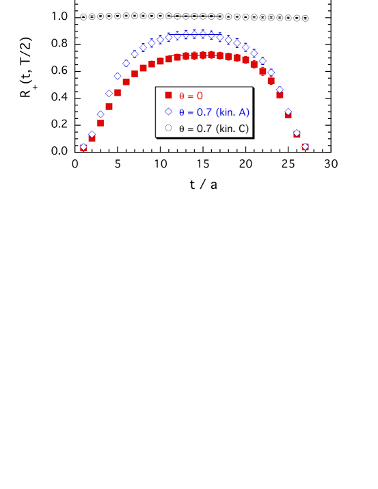
Fig. 2: Time dependence of the quantity $R_{+}(t_{x}=t,t_{y}=T/2)$ providing at large time distances the vector form factor $f_{+}(q^{2})$ (see footnote 3 in the text), calculated with periodic BCs ($\theta=0$) at $a^{2}q^{2}=-0.067$ (full squares), and with twisted BCs ($\vec{\theta}=(0.7,0,0)$) at $a^{2}q^{2}=-0.034$ in kinematics A (open diamonds) and $a^{2}q^{2}=0.0022$ in kinematics C (open dots). The plateaux are taken from $t/a=11$ to $t/a=17$. The values of the hopping parameters are $k_{s}=0.1349$ and $k_{\ell}=0.1339$.

In Fig. 3 our results for the form factors $f_{+}(q^{2})$ and $f_{0}(q^{2})$, obtained at $k_{s}=0.1349$ and $k_{\ell}=0.1339$ for the three kinematics A, B and C as well as for $\theta=0$, are reported, while in Fig. 4 the relative statistical errors, $\Delta f_{+}(q^{2})/f_{+}(q^{2})$ and $\Delta f_{0}(q^{2})/f_{0}(q^{2})$, are shown. It can be seen that the use of twisted BCs allows to explore the low-$q^{2}$ region without introducing any significant additional noise.

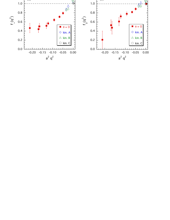
Fig. 3: Results for the form factors $f_{+}(q^{2})$ (a) and $f_{0}(q^{2})$ (b) obtained for various values of $q^{2}$ at $k_{s}=0.1349$ and $k_{\ell}=0.1339$. Full squares correspond to $\theta=0$, while open diamonds, triangles and dots correspond to the three kinematics A, B and C, respectively.

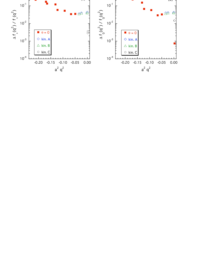
Fig. 4: As in Fig. 3 but for the relative statistical errors $\Delta f_{+}(q^{2})/f_{+}(q^{2})$ (a) and $\Delta f_{0}(q^{2})/f_{0}(q^{2})$ (b).

The statistical error of the results obtained at $\theta=0$ quickly decreases as $q^{2}$ increases in the space-like region, reaching a minimum value of $\simeq 3\%$ at $a^{2}q^{2}\simeq=-0.05$ for both $f_{+}(q^{2})$ and $f_{0}(q^{2})$. The results obtained using kinematics A and B are totally consistent with each other and the statistical error remains almost constant ($\simeq 4\%$). Note that the precision obtained in kinematics A and B is not better than the one of the nearest points obtained at $\theta=0$.

Vice versa a significant improvement in the precision can be achieved using kinematics C thanks to the double ratio (28), which allows to determine $f_{+}(q^{2})$ with a statistical error of $\simeq 0.3\%$. For the scalar form factor the corresponding accuracy is only $\simeq 1.5\%$ due to the larger fluctuations of the ratio (25), but it is still better than the precision achieved with kinematics A and B. The smallest statistical uncertainty ($\simeq 0.07\%$) remains the one at $q^{2}=q_{\rm max}^{2}$ thanks to the double ratio (24) that involves the time component of the weak vector current with all mesons at rest.

5 Slopes of $f_{+}(q^{2})$ and $f_{0}(q^{2})$ at $q^{2}=0$

In this Section we analyze the momentum dependence of the vector and scalar $K\to\pi$ form factors in order to understand the impact of the introduction of the twisted BCs in the determination of the form factors as well as of their slopes at zero-momentum transfer. As already noted in Ref. [3] the results for $f_{+}(q^{2})$ can be very well described by a pole-dominance fit, where the slope agrees well with the inverse of the $K^{*}$-meson mass square for each combination of the simulated quark masses. The results for $f_{0}(q^{2})$ can be parameterized using different functional forms, like the ones adopted in Ref. [3]. However, for our purposes it suffices to consider the case of a polar fit for both $f_{+}(q^{2})$ and $f_{0}(q^{2})$. We have checked that our final findings remain unchanged if instead of a polar fit a linear or quadratic $q^{2}$-dependence for $f_{0}(q^{2})$ is considered.

Thus our results have been parameterized using the following momentum dependencies

$$f_{+}(q^{2}) = \frac{f(0)}{1-\lambda_{+}~{}q^{2}}~{},$$

$$f_{0}(q^{2}) = \frac{f(0)}{1-\lambda_{0}~{}q^{2}}~{},$$ (30)

where $f(0)=f_{+}(0)=f_{0}(0)$, $\lambda_{0}$ and $\lambda_{+}$ are fitting parameters. We have determined the values of such three parameters through a $\chi^{2}$-minimization procedure applied to different sets of lattice data, namely: i) data obtained using periodic BCs only ($\theta=0$); ii) addition of the results corresponding to kinematics A and B; iii) data at $\theta=0$ plus those corresponding to kinematics C only; iv) full set of lattice points ($\theta=0$ plus kinematics A, B and C). In Table 2 we have reported the values obtained for $f(0)$, $\lambda_{0}$ and $\lambda_{+}$ for each choice of the data set. It can be seen that the impact of the lattice points corresponding to twisted BCs appears to be marginal and the extracted values of $f(0)$, $\lambda_{0}$ and $\lambda_{+}$ have almost the same accuracy as the one obtained using simply the lattice data calculated with periodic BCs. The usefulness of the twisted BCs is thus spoiled by the absence of a significant improvement of the accuracy as well as by the non-negligible increase of the computational time required for the inversions of Eq. (7) for each choice of $\vec{\theta}$.

lattice data set	$f(0)$	$\lambda_{0}/a^{2}$	$\lambda_{+}/a^{2}$
$\theta=0$	0.9907(19)	3.2(5)	5.9(8)
$\theta=0~{}+$ kin. A, B	0.9920(17)	2.8(5)	5.6(7)
$\theta=0~{}+$ kin. C	0.9910(16)	3.1(5)	6.0(8)
$\theta=0~{}+$ kin. A, B, C	0.9921(15)	2.7(4)	5.6(7)

Table 2: Values of the vector form factor at zero-momentum transfer $f(0)=f_{+}(0)=f_{0}(0)$ and of the slope parameters $\lambda_{0}$ and $\lambda_{+}$ of the polar fits (30), obtained using different sets of values of $f_{+}(q^{2})$ and $f_{0}(q^{2})$, including always the very accurate value of $f_{0}(q^{2})$ at $q^{2}=q_{\rm max}^{2}$. The values of the hopping parameters are $k_{s}=0.1349$ and $k_{\ell}=0.1339$.

This finding can be traced back to the following facts: i) the presence of the very accurate value of $f_{0}(q^{2})$ at $q^{2}=q_{\rm max}^{2}$ in all the data sets considered (such a data point is by far the most accurate one [see the rightmost point in Fig. 4(b)] and also the values of $q_{\rm max}^{2}$ are quite small [see Table 1]); and ii) the use of twisted BCs does not lead to a sufficient improvement of the precision with respect to the nearest space-like points obtained with periodic BCs.

As mentioned in the Introduction, there are cases of phenomenological interest where a lattice point at zero-momentum transfer is not accessible with periodic BCs. An important example is represented by some of the form factors entering hyperon semileptonic decays, like the weak magnetism, the weak electricity, the induced scalar and pseudoscalar form factors [6]. Thus, in order to clarify the role played by the $\vec{\theta}\neq 0$ lattice points, we have repeated the fitting procedure for the same lattice data sets but excluding always the very accurate value $f_{0}(q_{\rm max}^{2})$. This analysis is expected to be representative of the cases where a precise lattice point close to or at zero-momentum transfer is not accessible. Our results are reported in Table 3.

lattice data set	$f(0)$	$\lambda_{0}/a^{2}$	$\lambda_{+}/a^{2}$
$\theta=0$	1.107(105)	5.2(2.1)	8.1(2.4)
$\theta=0~{}+$ kin. A, B	1.089 (47)	4.7(8)	7.7(9)
$\theta=0~{}+$ kin. C	0.9934(23)	3.3(6)	6.0(8)
$\theta=0~{}+$ kin. A, B, C	0.9966(25)	3.0(5)	5.5(7)

Table 3: The same as in Table 2 but excluding in the data sets the value of $f_{0}(q^{2})$ at $q^{2}=q_{\rm max}^{2}$.

The following comments are in order:

• using the data set $\theta=0$ (only periodic BCs) the values of $f(0)$ and of the slopes are now more poorly determined. The statistical uncertainties turn out to be $\simeq 10\%$, $\simeq 40\%$ and $\simeq 30\%$ for $f(0)$, $\lambda_{0}$ and $\lambda_{+}$, respectively. Note that the accuracy obtained for $f(0)$ is almost $3$ times the precision of the nearest space-like points ($\simeq 3\%$);

• the accuracy improves by a factor of $\simeq 2$ when the data corresponding to kinematics A and B are included. Note that the accuracy of $f(0)$ is now comparable to the one of the $\vec{\theta}\neq 0$ points ($\simeq 4\%$), due to the fact that the latter are quite close to $q^{2}=0$. Clearly the $\simeq 5\%$ precision achieved for $f(0)$ is not enough for phenomenological applications to the $K_{\ell 3}$ decay. However such a level of accuracy is highly desirable for other observables, like hyperon semileptonic form factors;

• the inclusion of the quite accurate points obtained in kinematics C (with or without those of kinematics A and B) leads to a remarkably good determination of $f(0)$ and the slopes $\lambda_{0}$ and $\lambda_{+}$, obtaining a precision competitive with that reported in Table 2, where the very precise value $f_{0}(q_{\rm max}^{2})$ is included.

We have also performed the analysis of our lattice simulations at $k_{s}=0.1339$ and $k_{\ell}=0.1349$. The results obtained are similar to the ones shown in Figs. 2-4 and in Tables 2-3. Our findings about the impact of the twisted BCs remain unchanged. The same is true also for the $K\to K$ and $\pi\to\pi$ transitions, where $q_{\rm max}^{2}$ vanishes, $f_{-}(q^{2})=0$ and $f(0)=1$ because of vector current conservation. Note that for degenerate transitions, like the ones needed for the nucleon magnetic and the neutron electric dipole form factors, the kinematics A and B precisely coincide, while the kinematics C does not add any new information.

We mention that there are other cases of phenomenological interest where a lattice point at zero-momentum transfer is not accessible with periodic BCs. For instance the nucleon magnetic form factor $G_{M}(q^{2})$ is related to the matrix elements of the spatial components of the electromagnetic current, which are proportional to the value of the momentum transfer. Therefore, the nucleon magnetic moment $G_{M}(q^{2}=0)$ is not directly accessible with periodic BCs and it should be determined by a “long” extrapolation to $q^{2}=0$ (see Ref. [10]). Another example is the neutron electric dipole moment as determined with the strategies described in Refs. [11, 12], which require again a long extrapolation of the $CP$-violating neutron form factor $F_{3}(q^{2})$ to $q^{2}=0$ . In such cases however the introduction of twisted BCs is not trivial, because the current involved, the electromagnetic one, is not flavor changing. One can speculate that, by introducing an additional flavor and suitable interpolating fields, the application of the twisted BCs to the additional flavor, at least for quenched simulations, might provide the form factor of interest at quite small values of the four-momentum transfer. The application of twisted BCs to electromagnetic transitions requires therefore a careful treatment, which is well beyond the scope of the present work.

6 Conclusions

We have investigated the application of twisted boundary conditions to quenched lattice QCD simulations of three-point correlation functions in order to access spatial components of hadronic momenta different from the integer multiples of $2\pi/L$. The vector and scalar form factors relevant to the $K\to\pi$ semileptonic decay have been evaluated by twisting in all possible ways one of the quark lines in the three-point functions. We have found that the momentum shift produced by the twisted boundary conditions does not introduce any additional noise and easily allows to determine within a few percent statistical accuracy the form factors at quite small values of the four-momentum transfer, which are not accessible when periodic boundary conditions are considered. We are confident that these findings are independent of the use of the quenched approximation, so that they will hold as well also in case of partially quenched and full QCD simulations.

We have studied the impact of twisted boundary conditions on the precision of the determination of the $K\to\pi$ form factors and their slopes at zero momentum transfer. We have found that:   i) when the precise lattice point for $f_{0}(q^{2})$ at $q^{2}=q_{\rm max}^{2}$ is not included in the analysis, the use of twisted BCs is crucial to allow a determination of the form factor at zero-momentum transfer at a few percent statistical level;   ii) when the very accurate value $f_{0}(q_{\rm max}^{2})$ is included in the analysis, the impact of twisted BCs turns out to be marginal, while we remind it is expensive for the computational time. The latter result is due to the fact that:   i) the precision of the lattice points obtained with twisted BCs is not comparable to the one that can be achieved for $f_{0}(q_{\rm max}^{2})$;   ii) the use of twisted boundary conditions does not lead to a sufficient improvement of the precision with respect to the nearest points obtained with periodic boundary conditions.

We stress that there are cases of phenomenological interest where a lattice point at zero-momentum transfer is not accessible with periodic BCs, like e.g. the case of the weak magnetism, the weak electricity, the induced scalar and pseudoscalar form factors entering hyperon semileptonic decays.

References

• [1] P. F. Bedaque, Phys. Lett. B 593 (2004) 82 [arXiv:nucl-th/0402051].
• [2] G. M. de Divitiis, R. Petronzio and N. Tantalo, Phys. Lett. B 595 (2004) 408 [arXiv:hep-lat/0405002].
• [3] D. Becirevic et al., Nucl. Phys. B 705 (2005) 339 [arXiv:hep-ph/0403217] and Nucl. Phys. Proc. Suppl.  140 (2005) 387. See also for hyperon semileptonic decays: D. Becirevic et al., Eur. Phys. J. A 24S1 (2005) 69 [arXiv:hep-lat/0411016].
• [4] C. Dawson, T. Izubuchi, T. Kaneko, S. Sasaki and A. Soni, PoS LAT2005 (2005) 337 [arXiv:hep-lat/0510018]. N. Tsutsui et al. [JLQCD Collaboration], PoS LAT2005 (2005) 357 [arXiv:hep-lat/0510068].
• [5] M. Okamoto [Fermilab Lattice Collaboration], arXiv:hep-lat/0412044.
• [6] D. Guadagnoli, V. Lubicz, M. Papinutto and S. Simula, preprint RM3-TH/06-7.
• [7] C. T. Sachrajda and G. Villadoro, Phys. Lett. B 609 (2005) 73 [arXiv:hep-lat/0411033]. J. M. Flynn, A. Juttner and C. T. Sachrajda [UKQCD Collaboration], Phys. Lett. B 632 (2006) 313 [arXiv:hep-lat/0506016].
• [8] P. F. Bedaque and J. W. Chen, Phys. Lett. B 616 (2005) 208 [arXiv:hep-lat/0412023].
• [9] G. Martinelli and C. T. Sachrajda, Nucl. Phys. B 316 (1989) 355.
• [10] M. Gockeler et al. [QCDSF Collaboration], Phys. Rev. D 71 (2005) 034508 [arXiv:hep-lat/0303019].
• [11] E. Shintani et al., Phys. Rev. D 72 (2005) 014504 [arXiv:hep-lat/0505022].
• [12] F. Berruto, T. Blum, K. Orginos and A. Soni, Phys. Rev. D 73 (2006) 054509 [arXiv:hep-lat/0512004].
• [13] D. Guadagnoli, V. Lubicz, G. Martinelli and S. Simula, JHEP 0304 (2003) 019 [arXiv:hep-lat/0210044]. D. Guadagnoli and S. Simula, Nucl. Phys. B 670 (2003) 264 [arXiv:hep-lat/0307016].