String breaking

Abstract

We numerically investigate the transition of the static quark-antiquark string into a static-light meson-antimeson system. Improving noise reduction techniques, we are able to resolve the signature of string breaking dynamics for $n_{f}=2$ lattice QCD at zero temperature. We discuss the lattice techniques used and present results on energy levels and mixing angle of the static two-state system. We visualize the action density distribution in the region of string breaking as a function of the static colour source-antisource separation. The results can be related to properties of quarkonium systems.

1 INTRODUCTION

The breaking of the colour-electric string between two static sources is a prime example of a strong decay in QCD [1]. Recently, we reported on an investigation of this two state system [2, 3, 4], with a wave function $|Q\rangle$ created by a $\overline{Q}Q$ operator and a wave function $|B\rangle$ created by a four-quark $B\overline{B}$ operator, where $B=\overline{Q}q$. $Q$ denotes a static source and $q$ is a light quark.

We determined the energy levels $E_{1}(r)-2m_{B}$ and $E_{2}(r)-2m_{B}$ of the two physical eigenstates $|1\rangle$ and $|2\rangle$ which we decomposed into the components,

$$|1\rangle = \cos{\theta}\,|Q\rangle+\sin{\theta}\,|B\rangle$$ (1)

$$|2\rangle = -\sin{\theta}\,|Q\rangle+\cos{\theta}\,|B\rangle.$$ (2)

We characterise string breaking by the distance scale $r_{c}$ at which $\Delta E=E_{2}-E_{1}$ is minimized and by the energy gap $\Delta E_{c}=\Delta E(r_{c})$. While these energy levels and $r_{c}$ are first principles QCD predictions, the mixing angle $\theta$ is (slightly) model dependent: within each (Fock) sector there are further radial and gluonic excitations and we truncated the basis after the four quark operator.

In order to obtain dynamical information on the string breaking mechanism, we are studying the spatial energy and action density distributions within the two state system. In doing so one can address questions about the localisation of the light $q\bar{q}$ pair that is created when $r$ is increased beyond $r_{c}$. The energy density will decrease fastest in those places where $q\bar{q}$ creation is most likely. Perturbation theory suggests that light pair creation close to one of the static sources is favoured by the Coulomb energy gain while aesthetic arguments might suggest a symmetric situation with $q\bar{q}$ dominantly being created near the centre. First results on this investigation are presented here.

2 PARAMETERS AND METHODS

We use $n_{f}=2$ Wilson fermions at a quark mass slightly smaller than the physical strange quark and a lattice spacing $a=0.166(2)\,r_{0}\approx 0.083(1)$ fm and find [3], $r_{c}=2.5(3)\,r_{0}\approx 1.25(1)\,\mbox{fm}$ and $\Delta E_{c}\approx 51(3)$ MeV, where the errors do not include the phenomenological uncertainty of assigning a physical scale to $r_{0}\approx 0.5$ fm. Using data on the $\overline{Q}Q$ potential and the static-light meson mass $m_{B}$, obtained at different quark masses, we determine the real world estimate, $r_{c}=1.13(10)(10)$ fm, where the errors reflect all systematics. An extrapolation of $\Delta E_{c}$ however is impossible, without additional simulations at lighter quark masses.

These results became possible by combining a variety of improvement techniques: the necessary all-to-all light quark propagators were calculated from the lowest eigenmodes of the Wilson-Dirac operator, multiplied by $\gamma_{5}$, after a variance reduced stochastic estimator correction step. The signal was improved by employing a fat link static action. Many off-axis distances were implemented to allow for a fine spatial resolution of the string breaking region. For details see Ref. [3].

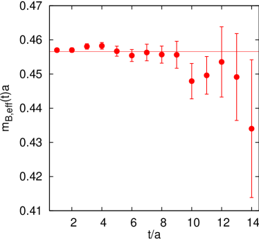
Figure 1: Static-light effective masses, $am_{B,\mbox{eff}}=\ln[C_{B}(t)/C_{B}(t+a)]$, where $C_{B}(t)$ is the static-light mesonic correlation function.

Great care was also spent on optimizing the overlap with the ground states, within the $|Q\rangle$ and $|B\rangle$ sectors, using combinations of APE [5, 6] and Wuppertal [7] smearing. Our APE smearing consists of the replacement,

$$U_{x,i}^{(n+1)}=P_{SU(3)}\left(\alpha\,U_{x,i}^{(n)}+\Sigma_{x,i}^{(n)}\right).$$ (3)

$P_{SU(3)}$ denotes a projection operator, back onto the $SU(3)$ group, and

$$\Sigma_{x,i}^{(n)}=\sum_{|j|\neq i}U_{x,j}^{(n)}U^{(n)}_{x+a\hat{\boldsymbol{\jmath}},i}U^{(n)\dagger}_{x+a\hat{\boldsymbol{\imath}},j},$$ (4)

$i\in\{1,2,3\},j\in\{\pm 1,\pm 2,\pm 3\}$, is the spatial staple-sum, surrounding $U_{x,i}^{(n)}$. We choose $\alpha=2.0$ and define our APE smeared links, $\widetilde{U}_{x,i}=U_{x,i}^{(50)}$. For the projection we use,

$$P_{SU(3)}(A) = A^{\prime}\det(A^{\prime})^{-1/3}\in SU(3),$$

$$A^{\prime} = \frac{A}{\sqrt{A^{\dagger}A}}\in U(3).$$ (5)

The spatial transporters within our $\overline{Q}Q$ states are products of APE smeared links, taken along the shortest lattice distance between the two sources. The APE smeared links are also employed for the parallel transport within the Wuppertal smearing of light quark sources, used to improve the static-light meson operators:

$$\phi^{(n+1)}_{x}=\frac{1}{1+6\delta}\left(\phi^{(n)}_{x}+\delta\sum_{j=\pm 1}^{\pm 3}\widetilde{U}_{x,j}\phi^{(n)}_{x+a\hat{\boldsymbol{\jmath}}}\right).$$ (6)

We set $\delta=4$ and take the linear combination $\phi^{(20)}-6.6323\phi^{(40)}+7.2604\phi^{(50)}$ as our smearing function. Best results are obtained by using smeared-local quark propagators. The quality of the overlap with the static-light mesonic ground state is visualized in the effective mass plot Figure 1. Note that we display the effective masses up to physical distances $t>1.2$ fm.

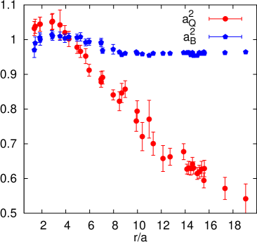
Figure 2: The overlaps of our test wave functions with the $|Q\rangle$ and $|B\rangle$ Fock states. String breaking takes place around $r_{c}\approx 15\,a$.

We were able to achieve values of $|a_{Q}|^{2}=|\langle\Psi_{Q}|Q\rangle|^{2}=0.62(2)$ and $|a_{B}|^{2}=|\langle\Psi_{B}|B\rangle|^{2}=0.96(1)$ at $r\approx r_{c}$ for the overlaps of our test wave functions $|\Psi_{X}\rangle$ with the respective states on the right hand sides of Eqs. (1) and (2). We display these results in Figure 2. The almost optimal value $|a_{B}|\approx 1$ was essential to allow $E_{1}$, $E_{2}$ and $\theta$ to be fitted from correlation matrix data,

$$C(t) = \left(\begin{array}[]{cc}C_{QQ}(t)&C_{QB}(t)\\ C_{BQ}(t)&C_{BB}(t)\end{array}\right)$$ (9)

$$= \left(\begin{array}[]{cc}\mbox{ \begin{minipage}{16.0pt}\includegraphics[width=16.0pt]{w11.ps}\end{minipage}}&\sqrt{n_{f}}\mbox{ \begin{minipage}{16.0pt}\includegraphics[width=16.0pt]{w12.ps}\end{minipage}}\\ &\\ \sqrt{n_{f}}\mbox{ \begin{minipage}{16.0pt}\includegraphics[width=16.0pt]{w21.ps}\end{minipage}}&-n_{f}\mbox{ \begin{minipage}{16.0pt}\includegraphics[width=16.0pt]{w22c.ps}\end{minipage}}+\mbox{ \begin{minipage}{16.0pt}\includegraphics[width=16.0pt]{w22d.ps}\end{minipage}}\end{array}\right),$$ (13)

obtained at moderate Euclidean times: $t\geq 2a$ for $C_{BB}$ and $t\geq 4a$ for the remaining 2 matrix elements $C_{QQ}$ and $C_{QB}=C_{BQ}$ at $r\approx r_{c}$.

We follow Ref. [8] and define action and energy density distributions,

$$\sigma_{n}({\mathbf{x}})=\frac{1}{2}\left[{\mathcal{E}}_{n}({\mathbf{x}})+{\mathcal{B}}_{n}({\mathbf{x}})\right],$$ (14)

$$\epsilon_{n}({\mathbf{x}})=\frac{1}{2}\left[{\mathcal{E}}_{n}({\mathbf{x}})-{\mathcal{B}}_{n}({\mathbf{x}})\right],$$ (15)

where

$${\mathcal{A}}_{n}({\mathbf{x}}) = \langle n|A^{2}({\mathbf{x}})|n\rangle-\langle A^{2}\rangle$$

$$= \lim_{t\rightarrow\infty}\frac{\langle\Phi_{n}(t)|A^{2}({\mathbf{x},t/2})|\Phi_{n}(0)\rangle}{\langle\Phi_{n}(t)|\Phi_{n}(0)\rangle}-\langle A^{2}\rangle$$

$\Phi_{n}$ are our approximations to the creation operators of the states $|n\rangle$, obtained from the diagonalisation of $C(t)$. We have suppressed the distance $r$ from the above formulae and $n=1$ denotes the ground state (dominantly $\overline{Q}Q$ at $r<r_{c}$) and $n=2$ the excitation (dominantly $B\overline{B}$ at $r<r_{c}$). Electric and magnetic fields are calculated from the plaquette,

$$E^{2}\left(x+\frac{a}{2}\hat{\mathbf{4}}\right)=\frac{\beta}{a^{4}}\sum_{i=1}^{3}\left[\overline{U}_{x,i4}+\overline{U}_{x-a\hat{\boldsymbol{\imath}},i4}\right],$$ (17)

$$B^{2}(x)=\frac{\beta}{2a^{4}}\sum_{i=1}^{3}\!\!\!\!\!\!\!\! \left[\overline{U}_{x,ij}(x)+\overline{U}_{x-a\hat{\boldsymbol{\imath}},ij}\right.$$

$$\left.+\overline{U}_{x-a\hat{\boldsymbol{\jmath}},ij}+\overline{U}_{x-a(\hat{\boldsymbol{\imath}}+\hat{\boldsymbol{\jmath}}),ij}\right],$$

where $j=\mbox{mod}(i,3)+1$ and,

$$\overline{U}_{x,\mu\nu}=\frac{z_{0}}{3}\mbox{tr}\,\left(\overline{U}_{x,\mu}\overline{U}_{x+a\hat{\boldsymbol{\mu}},\nu}\overline{U}^{\dagger}_{x+a\hat{\boldsymbol{\nu}},\mu}\overline{U}^{\dagger}_{x,\nu}\right).$$ (19)

We implement two different operators with the same continuum limits: in one case we identify $\overline{U}_{x,\mu}$ with the link $U_{x,\mu}$ connecting $x$ with $x+a\hat{\boldsymbol{\mu}}$. Additionally, we used smeared operators,

$$\overline{U}_{x,\mu}=P_{SU(3)}\left(\gamma\,U_{x,\mu}+\Sigma^{\prime}_{x,\mu}\right),$$ (20)

where $\gamma=0.4$ and $\Sigma^{\prime}_{x,\mu}$ is the sum over all six staples enclosing $U_{x,\mu}$, in the three forward and in the three backward directions. The $\gamma$-value was tuned to maximize the average plaquette, calculated from the smeared links. For the un-smeared plaquette $z_{0}=1$ in Eq. (19) while for smeared plaquettes $z_{0}=1+O(\alpha_{s})$ is adjusted such that the vacuum expectation value of the average plaquette remains unchanged.

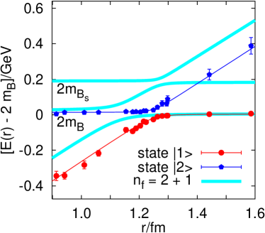
Figure 3: The energy levels in physical units for $n_{f}=2$. The bands represent the expected $n_{f}=2+1$ scenario.

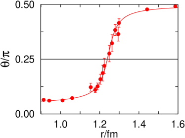
Figure 4: The mixing angle $\theta$.

The plaquette smearing enhances the signal/noise ratio. Due to this smearing and the fat link static action used, the peaks of the distributions around the source positions (that will diverge in the continuum limit) are less singular than in previous studies of $SU(2)$ gauge theory at similar lattice spacings [8]. In the continuum limit the results from smeared and un-smeared plaquette probes will coincide, away from these self energy peaks. The draw back of plaquette smearing is that exact reflection positivity is violated. However, our wave functions are sufficiently optimized to compensate for this.

We insert the $E^{2}({\mathbf{x}},t)$ and $B^{2}({\mathbf{x}},t)$ operators at position $t/2$ into the correlation matrix $C(t)$, Eq. (9). For even$|$odd $t/a$-values we average $E^{2}|B^{2}$ over the two adjacent time slices, respectively. Using the fitted ground state overlap ratio $a_{Q}/a_{B}$ and the mixing angle $\theta$ as inputs, we calculate the action and energy density distributions Eqs. (14) and (15) in the limit of large $t$ via Eq. (2) from the measured matrix elements. The distributions agree within errors within the time range $3a\leq t\leq 6a$. The results presented here are based on our $t=4a$ analysis.

3 RESULTS

To set the stage, we display the main results of Ref. [3] in Figures 3 and 4. In the first figure we also speculate about the scenario in the real world with possible decays into $B\overline{B}$ as well as into $B_{s}\overline{B}_{s}$. For our parameter settings and $n_{f}=2$ string breaking occurs at a distance $r_{c}\approx 1.25$ fm. In Figure 4 we show the mixing angle as a function of the distance. The $B\overline{B}$ content of the ground state is given by $\sin\theta$. Within our statistical errors $\theta$ reaches $\pi/4$ at $r=r_{c}$. Remarkably, there is a significant four quark component in the ground state at $r<r_{c}$ while for $r>r_{c}$ the limit $\theta\rightarrow\pi/2$ is rapidly approached.

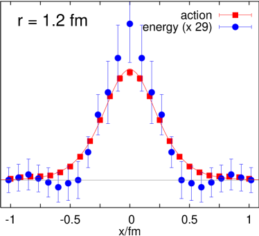
Figure 5: The transverse profile in the centre of the flux tube.

Our basis vectors $|Q\rangle$ and $|B\rangle$ are no eigenstates of the system. The transition rate, $g\propto dC_{QB}/dt$, can be related to energy gap and mixing angle: $g(r)\approx\Delta E(r)\sin(\theta)\cos(\theta)$. This means that $\Delta E_{c}\approx 2g(r)$. With a transition rate of only about 25 MeV in the string breaking region and even smaller $g(r)$-values at $r>r_{c}$, a detection of the ground state contribution to the standard Wilson loop at $r>r_{c}$, where $|1\rangle$ contains little $|Q\rangle$ admixture, is hopeless: one would have to resolve the correlation function at times of order $1/g\approx 8$ fm! For a complementary view on the problem, in the context of the breaking of higher representation strings in pure gauge theories, see e.g. Ref. [9].

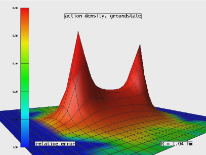
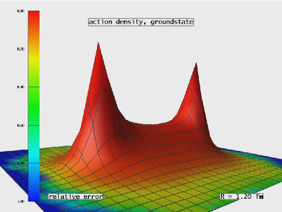
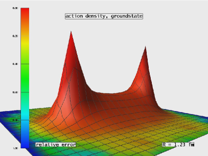
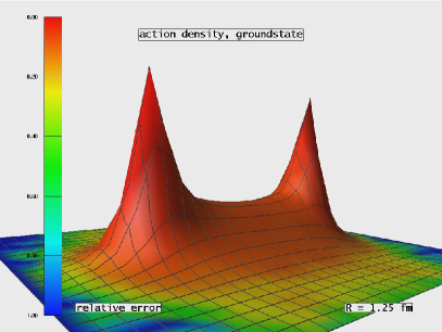
Figure 6: Ground state action density distribution at $r\leq r_{c}$.

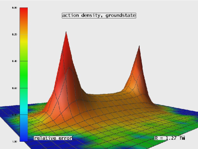
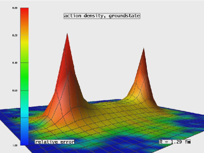
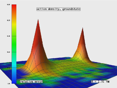
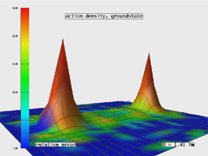
Figure 7: Ground state action density distribution at $r>r_{c}$.

Diagrammatically, $g(r)$ can be represented as,

$$g(r)=\frac{n_{f}\mbox{ \begin{minipage}{16.0pt}\includegraphics[width=16.0pt]{w12.ps}\end{minipage}}}{\left(\mbox{ \begin{minipage}{16.0pt}\includegraphics[width=16.0pt]{w11.ps}\end{minipage}}\times n_{f}^{2}\mbox{ \begin{minipage}{16.0pt}\includegraphics[width=16.0pt]{w22d.ps}\end{minipage}}\right)^{1/2}}\propto\sqrt{\frac{n_{f}}{N_{c}}},$$ (21)

where $N_{c}$ is the number of colours: the large $N_{c}\gg n_{f}$ expectation for the minimal energy gap is, $\Delta E_{c}\propto\sqrt{n_{f}/N_{c}}$. Obviously, precision studies at different $N_{c}$ and $n_{f}$ are needed to establish the validity range of this prediction. The decay of the adjoint potential into two gluelumps, where $\Delta E_{c}\propto 1/N_{c}$, also fits nicely into this context.

The quality of our density distribution data is depicted in Figure 5 for the ground state at a separation slightly smaller than $r_{c}$, as a function of the transverse distance $x$ from the $\overline{Q}Q$ axis. Due to cancellations between the magnetic and electric components the energy density is much smaller than the action density: for the comparison we have multiplied the energy density data by the arbitrary factor of 29. Note that the ratio $\sigma/\epsilon$ will diverge like $-\ln a\Lambda$ in the continuum limit. The differences between the shapes of the energy and action density distributions are not statistically significant. Below we only visualise the more precise action density results.

We employ several off-axis separations. Assuming rotational symmetry about the interquark axis, each point is labelled by two coordinates. $x$ denotes the distance from the $\overline{Q}Q$ axis and $y$ denotes the longitudinal distance from the centre point. We define an interpolating rectangular grid with perpendicular lattice spacing $a$ and the longitudinal spacing slightly scaled, such that the static sources always lie on integer grid coordinates. We then assign a quadratically interpolated value to each grid point ${\mathbf{z}}$, obtained from points in the neighbourhood, $|{\mathbf{z}}-(x,y)|\leq\epsilon=a$. On the axis the data points are more sparse and we relax the condition to $\epsilon=\sqrt{3}a$ while for the singular peaks we maintain the un-interpolated values.

In Figures 6 and 7 we display ground state action density distributions for different distances around $r_{c}$. An mpeg animation has been published in Ref. [4]. The colour encodes the relative statistical errors and the lattice mesh represents our spatial resolution $a$. As already evident from the mixing angle $\theta(r)$ of Figure 4 above, string breaking takes place within a small region around $r_{c}$. All distributions are very similar to linear superpositions of string and broken-string states, with no non-trivial spatial dependence: string breaking appears to resemble an instantaneous process, without evidence of localisation of the $q\bar{q}$ pair creation.

4 APPLICATION TO QUARKONIUM DECAY

We wish to relate the static limit results to strong decay rates of quarkonia. In the non-relativistic limit of heavy quarks, potential “models” provide us with the natural framework for such studies. In fact at short distances, $r\ll 1/\Lambda$, potential “models” can be derived as an effective field theory, potential NRQCD, from QCD [10]. One can in principle add a $B\overline{B}$ sector, as well as transition terms between the two sectors, to the $\overline{Q}Q$ pNRQCD Lagrangian. Strong decays would then be a straightforward non-perturbative generalisation of the standard multipole treatment of radiative transitions in QED. Unfortunately, transitions such as $\Upsilon(4S)\rightarrow B\overline{B}$ can hardly be classed as “short distance” physics. So, some modelling is required instead.

The natural starting point again is a two channel potential model which might still have some validity beyond the short distance regime:

$$H\psi({\mathbf{r}})=E\psi({\mathbf{r}})$$ (22)

with

$$H=\left(\begin{array}[]{cc}\frac{1}{m_{Q}}&0\\ 0&\frac{1}{m_{B}}\end{array}\right){\mathbf{p}}^{2}+V(r).$$ (23)

$m_{Q}$ denotes the heavy quark mass and $m_{B}$ is the mass of a $B$ meson. The wavefunction has two components,

$$\psi({\mathbf{r}})=\left(\begin{array}[]{c}\psi_{\overline{Q}Q}({\mathbf{r}})\\ \psi_{B\overline{B}}({\mathbf{r}})\end{array}\right)$$ (24)

and the potential is given by,

$$V(r) = O^{\dagger}\left(\begin{array}[]{cc}E_{1}(r)&0\\ 0&E_{2}(r)\end{array}\right)O$$ (27)

$$= \left(\begin{array}[]{cc}E_{Q}(r)&g(r)\\ g(r)&E_{B}(r)\end{array}\right),$$ (30)

where we have normalized the zero point energy to $2m_{B}$ and

$$O=\left(\begin{array}[]{cc}\cos\theta&\sin\theta\\ -\sin\theta&\cos\theta\end{array}\right)$$ (31)

rotates our Fock basis $\{|Q\rangle,|B\rangle\}$ into the eigenbasis $\{|1\rangle,|2\rangle\}$. We neglect $B$-$\overline{B}$ interactions and set $E_{B}(r)=0$. We further adjust the difference $m_{\Upsilon(4S)}-2m_{B}$ to the experimental value which affects our phase space factor. We then follow Ref. [11] and calculate the decay rate by multiplying phase space with the overlap integral between the $\Upsilon(4S)$ wave function, the interaction term $g(r)$ and the $B\overline{B}$ continuum. In doing so, we assume that the interaction does not contain any spatial distribution but only depends on the distance $r$. This instantaneous picture is supported by our action density measurements above.

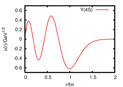
Figure 8: The radial $\Upsilon(4S)$ wave function.

In Figure 8 we display our radial $\Upsilon(4S)$ wave function $u(r)=\sqrt{4\pi}\,r\,\psi_{\overline{Q}Q,400}(r)$. The decay rate depends rather sensitively on the positions of the nodes. We obtain a preliminary result $\Gamma[\Upsilon(4S)\rightarrow B\overline{B}]\approx 5$ MeV, which is about half the experimental value. This appears very reasonable, given the crudeness of the model and the fact that the gap $\Delta E_{c}$ will increase with lighter, more realistic sea quark masses. We are studying the situation and systematics in more detail.

5 CONCLUSIONS

We were able to resolve the string breaking problem in $n_{f}=2$ QCD, at one value of the lattice spacing $a^{-1}\approx 2.37$ GeV and of the sea quark mass, $m\lesssim m_{s}$. It was also possible to study the dynamics of string breaking in detail and to resolve spatial colour field distributions. The breaking of the string appears to be an instantaneous process, with de-localized light quark pair creation. While a direct lattice study of strong decay rates such as $\Upsilon(4S)\rightarrow B\overline{B}$ or $\Psi(3S)\rightarrow\overline{D}D$ is at present virtually impossible, investigations in the static limit can help constraining models. Studying the energy between pairs of static-light mesons can also be viewed as a milestone with respect to future calculations of $\Lambda_{Q}\Lambda_{Q}$ forces, which are related to nucleon-nucleon interactions [12].

References

- [1] C. Michael, PoS LAT2005, 008 (2005) [arXiv:hep-lat/0509023].
- [2] G.S. Bali et al., arXiv:hep-lat/0409137.
- [3] G.S. Bali et al. [SESAM], Phys. Rev. D 71, 114513 (2005) [arXiv:hep-lat/0505012].
- [4] Z. Prkacin et al. PoS LAT2005, 308 (2005) [arXiv:hep-lat/0510051].
- [5] M. Albanese et al. [APE], Phys. Lett. 192B, 163 (1987).
- [6] M. Teper, Phys. Lett. 183B, 345 (1987).
- [7] S. Güsken et al., Phys. Lett. B 227, 266 (1989).
- [8] G.S. Bali, K. Schilling and C. Schlichter, Phys. Rev. D 51, 5165 (1995).
- [9] F. Gliozzi and A. Rago, Nucl. Phys. B 714, 91 (2005) [arXiv:hep-lat/0411004].
- [10] N. Brambilla, A. Pineda, J. Soto and A. Vairo, arXiv:hep-ph/0410047.
- [11] I.T. Drummond and R.R. Horgan, Phys. Lett. B 447, 298 (1999) [arXiv:hep-lat/9811016].
- [12] D. Arndt, S. R. Beane and M. J. Savage, Nucl. Phys. A 726, 339 (2003) [arXiv:nucl-th/0304004].