QCD with two dynamical flavors of chirally improved quarks

Abstract

Considering Ginsparg-Wilson type fermions dynamically in lattice QCD simulations is a challenging task. The hope is to be able to approach smaller pion masses and to eventually reach physical situations. The price to pay is substantially higher computational costs. Here we discuss first results of a dynamical implementation of the so-called Chirally Improved Fermions, a Dirac operator that obeys the Ginsparg-Wilson condition approximately. The simulation is for two species of mass-degenerate quarks on $12^{3}\times 24$ lattices with spatial size up to 1.55 fm. Implementation of the Hybrid Monte-Carlo algorithm and an analysis of the results are presented.

I Introduction

Quantum Chromodynamics (QCD) is a quantum field theory with a complicated vacuum structure, involving creation and annihilation of particle-antiparticle pairs in the vacuum. Presently the most promising approach for studying this theory non-perturbatively seems to be through Monte-Carlo simulations of the theory on a space-time lattice. Fermions, however, are described by Grassmann variables and have no simple representation appropriate for simulations. Fortunately the fermions occur bilinearly in the action and in the path integral the Grassmann integration can be performed explicitly. This leads to the fermion determinant as a weight factor. Each fermion species accounts for one such factor.

In lattice QCD Monte-Carlo simulations the path integral is approximated by averages over a finite set of configurations on a finite euclidian space-time grid. It is well understood how to sample gauge field configurations with the full dynamics of interacting gauge fields alone. It is a challenging task, however, to take into account the contribution of the fermion determinant in generating the probability measure. In the quenched approximation these determinants are put to unity by hand. Here we perform a simulation with full dynamical quarks, i.e., taking this determinant into account.

One of the crucial problems in putting fermions on the lattice is preserving their chiral symmetry. As an example consider the original Wilson Dirac operator. It exhibits spurious zero eigenvalues even at values of the fermionic mass parameter that correspond to non-zero pion masses. This feature complicates the approach to the chiral limit. On the other hand, Dirac operators obeying the Ginsparg-Wilson (GW) condition GiWi82 exactly, have no such spurious modes. However, the only known explicit and exact realization of such an operator, the so-called overlap operator NaNe93a95 ; Ne9898a is quite expensive to construct and implement in dynamical simulations FoKaSz0405 ; EgFoKa05 ; CuKrFr05 ; CuKrLi05 ; DeSc05a ; DeSc05b . Various other Dirac operators have been suggested, that fulfill the GW condition in an approximate way, among them the Domain Wall Fermions Ka92 ; FuSh95 ; AoBlCh04 ; AnBoBo05 , the Perfect Fermions HaNi94 ; HaHaNi05 or the Chirally Improved (CI) Fermions Ga01 ; GaHiLa00 . Such Ginsparg-Wilson-type fermions have the chance to allow a better approach to the chiral limit, i.e., to come closer to the physical value of the pion mass.

CI fermions have been extensively tested in quenched calculations (see, e.g., Ref. GaGoHa03a ). In these tests it was found that one can go to smaller quark masses without running into the problem of exceptional configurations. On quenched configurations pion masses down to 280 MeV could be reached on lattices of size $16^{3}\times 32$ (lattice spacing 0.148 fm) and about 340 MeV on $12^{3}\times 24$ lattices.

The challenge is to implement these fermions in dynamical, full QCD simulations. We discuss here such a simulation for two light, mass-degenerate flavors of dynamical quarks. For updating the gauge fields we use the standard Hybrid Monte-Carlo (HMC) algorithm. We report on our implementation of $D_{\textrm{\scriptsize{CI}}}$ for the HMC updating and present results of runs at lattice spacings in the range 0.11–0.13 fm for $12^{3}\times 24$ lattices of physical spatial extents of ${\cal O}(1.55\;\textrm{fm})$. Preliminary results on smaller lattices have been presented elsewhere LaMaOr05a ; LaMaOr05b .

II Algorithmic concerns

II.1 The Dirac operator and the action

The CI Dirac operator $D_{\textrm{\scriptsize{CI}}}$ was constructed by writing a general ansatz for the Dirac operator

$$D_{ij}=\sum_{k=1}^{16}\alpha^{k}_{ij}(U)\,\Gamma_{k}\;,$$ (1)

where $\Gamma_{k}$ $(k=1\ldots 16)$ are the 16 elements of the Clifford algebra and $\alpha^{k}_{ij}(U)$ are sums of path ordered products of links $U$ connecting lattice site $i$ with site $j$. Inserting $D$ into the GW relation and solving the resulting algebraic equations yields the CI Dirac operator $D_{\textrm{\scriptsize{CI}}}$. In principle this can be an exact solution, but that would require an infinite number of terms. In practice the number of terms is finite and the operator is a truncated series solution to the Ginsparg-Wilson relation, respecting the lattice symmetries, parity, invariance under charge conjugation as well as $\gamma_{5}$-hermiticity, but connecting sites only over a certain distance. For our implementation we use terms up to path lengths of four Ga01 ; GaHiLa00 .

Smearing is an essential quality improving ingredient in our Dirac operator. In the quenched studies for $D_{\textrm{\scriptsize{CI}}}$ GaGoHa03a it was found that smearing the gauge links was important (using HYP smearing HaKn01 ) as it resulted in better chiral properties for the operator, i.e., the spectrum showed less deviation from the Ginsparg-Wilson circle compared to the unsmeared case. Therefore we decided to use one level of smearing in our studies, too. Usual HYP smearing, however, is not well suited for use in HMC. The recent introduction of the differentiable “stout”-smearing MoPe04 opened the possibility to implement HMC for smeared fermionic actions. We thus used one level of isotropic stout smearing of the gauge configuration as part of the definition of the Dirac operator. Our smearing parameter ($\approx$ 0.165 in the notation of Ref. MoPe04 ) was chosen to maximize the plaquette value. A comparison between HYP and stout smearing on loops of different sizes on the same background has been presented in LaMaOr05b .

In quenched calculations Ga01 ; GaHiLa00 it was found that the tadpole improved Lüscher-Weisz LuWe85 gauge action had certain advantages over the Wilson gauge action in the sense that the configurations produced with this action were smoother than the ones produced by the Wilson gauge action. We therefore used this gauge action in our dynamical studies. It is given by

$$S_{g} = -\beta_{1}\sum_{\textrm{\scriptsize{pl}}}\frac{1}{3}\,\textrm{Re \,{tr}}\;U_{\textrm{\scriptsize{pl}}}-\beta_{2}\sum_{\textrm{\scriptsize{re}}}\frac{1}{3}\,\textrm{Re \,{tr}}\;U_{\textrm{\scriptsize{re}}}$$ (2)

$$-\beta_{3}\sum_{\textrm{\scriptsize{tb}}}\frac{1}{3}\,\textrm{Re \,{tr}}\;U_{\textrm{\scriptsize{tb}}}\;,$$

where $U_{\textrm{\scriptsize{pl}}}$ is the usual plaquette term, $U_{\textrm{\scriptsize{re}}}$ are Wilson loops of rectangular $2\times 1$ shape and $U_{\textrm{\scriptsize{tb}}}$ denote loops of length 6 along edges of 3-cubes (“twisted bent” or “twisted chair”). The coefficient $\beta_{1}$ is the independent gauge coupling and the other two coefficients $\beta_{2}$ and $\beta_{3}$ are determined from tadpole-improved perturbation theory. They have to be calculated self-consistently AlDiLe95 from

$$u_{0}=\left(\frac{1}{3}\,\textrm{Re \,$\textrm{tr}$}\langle U_{\textrm{\scriptsize{pl}}}\rangle\right)^{\frac{1}{4}}\;,\quad\alpha=-\frac{1}{3.06839}\,\log\left(u_{0}^{4}\right)\;,$$ (3)

as

$$\beta_{2}=\frac{\beta_{1}}{20\,u_{0}^{2}}\,(1+0.4805\,\alpha)\;,\quad\beta_{3}=\frac{\beta_{1}}{u_{0}^{2}}\,0.03325\,\alpha\;.$$ (4)

This determination should be done for each set of parameters $(\beta_{1},m)$.

Putting together all of the above, the partition function that we simulate assumes the form

$${\mathcal{Z}}=\int\,{\mathcal{D}}U\,{\mathcal{D}}\phi\,{\mathcal{D}}\phi^{{\dagger}}\;e^{-S_{g}-\phi^{{\dagger}}(M^{{\dagger}}M)^{-1}\phi}\;,$$ (5)

where $M$ denotes the massive Dirac operator given by

$$M(\overline{U},\,m)\equiv D_{\textrm{\scriptsize{CI}}}(m)\equiv D_{\textrm{\scriptsize{CI}}}(\overline{U})+{\bf 1}\,m\;,$$ (6)

$\overline{U}$ denotes the smeared link variable, and $\phi$ denotes the bosonic pseudofermion field.

II.2 HMC for CI fermions

The algorithm we used for our simulations is standard HMC DuKePe87 as this seems to be the most efficient one for simulating fermions at the moment. Although our implementation follows Ref. GoLiTo87 very closely, we believe that the additional complications due to the extended structure of our Dirac operator warrants some discussion.

HMC consists of a molecular dynamics (MD) evolution in $2\,n$ dimensional phase space (where $n$ is the original dimension of the theory) with simulation time as the evolution parameter. This involves introducing conjugate momenta and constructing a Hamiltonian for the problem. In our case, to construct a Hamiltonian, we introduce traceless hermitian matrices $p_{i,\mu}\in su(3)$ acting as momenta conjugate to the $U_{i,\mu}$ ($i$ being the site index and $\mu$ the direction of the link) and write

$$\mathcal{H}=\frac{1}{2}\sum_{i,\mu}\mathrm{tr}\left(p_{i,\mu}^{2}\right)+S_{g}+\phi^{\dagger}\left(M^{\dagger}\,M\right)^{-1}\phi\;.$$ (7)

There are two evolution equations for $U_{i,\mu}$ and $p_{i,\mu}$. While ${\dot{U}}_{i,\mu}=i\,p_{i,\mu}U_{i,\mu}$ , the equation for ${\dot{p}}_{i,\mu}$ is obtained by setting $\dot{\mathcal{H}}=0$,

$$0=\dot{\mathcal{H}}=\sum_{j,\mu}\,\mathrm{tr}\ p_{j,\mu}\,\dot{p}_{j,\mu}+\dot{S_{g}}+\phi^{{\dagger}}\,\frac{d}{dt}\left(M^{{\dagger}}M\right)^{-1}\,\phi\;.$$ (8)

Up to this point there is no difference to HMC with Wilson or staggered fermions. The first complication comes when we take the time derivative of our operator. Unlike Wilson or Staggered Dirac operators, which have only one link connecting the neighboring sites, we have longer paths.

As an example let us look at a path of length three. Let

$$\mathcal{U}=U_{j_{1},\mu_{1}}U^{\dagger}_{j_{2},\mu_{2}}U_{j_{3},\mu_{3}}\;.$$ (9)

Taking the time derivative, we find

$$\frac{d\,\mathcal{U}}{dt} = i\,p_{j_{1},\mu_{1}}\,U_{j_{1},\mu_{1}}U^{\dagger}_{j_{2},\mu_{2}}U_{j_{3},\mu_{3}}$$ (10)

$$+U_{j_{1},\mu_{1}}\,U^{\dagger}_{j_{2},\mu_{2}}(-i\,p_{j_{2},\mu_{2}})U_{j_{3},\mu_{3}}$$

$$+U_{j_{1},\mu_{1}}U^{\dagger}_{j_{2},\mu_{2}}(i\,p_{j_{3},\mu_{3}}U_{j_{3},\mu_{3}})\;,$$

where we have replaced ${\dot{U}}_{i,\mu}$ by $i\,p_{i,\mu}U_{i,\mu}$. The time derivative of the Dirac operator can thus be expressed as

$$\frac{dM}{dt}=\sum_{j,\mu,k}c_{j,\mu,k}W^{(1)}_{j,\mu,k}(\pm ip_{j,\mu})W^{(2)}_{j,\mu,k}\;,$$ (11)

where $W^{(1)}$ and $W^{(2)}$ contain products of links. To obtain our equation of motion for ${\dot{p}}_{j,\mu}$, we have to carefully cyclically permute the terms in $\phi^{{\dagger}}\frac{d}{dt}\left(M^{{\dagger}}M\right)^{-1}\phi$ until all the $p_{j,\mu}$ occur at the same position, at the front of the expression. This is of course required due to the non-Abelian nature of the variables and it is possible to cyclically permute them because we have an overall trace over both color and Dirac indices. In fact the trace on the Dirac indices can be carried out completely as the momenta and gauge part of the Hamiltonian do not have Dirac indices. The color trace on the other hand should not be carried out as we want an equation for the color matrices.

Finally our equation can be symbolically written in the form

$$p_{j,\mu}\,{\dot{p}}_{j,\mu}=-i\,p_{j,\mu}\sum(staples)_{j,\mu}-i\,p_{j,\mu}\sum(Dirac)_{j,\mu}\;.$$ (12)

From this we get our equation for ${\dot{p}}_{j,\mu}$. To ensure the group property for the link variables we actually take the traceless part of the r.h.s. of (12) for ${\dot{p}}_{j,\mu}$, as usual.

Since the $D_{\textrm{\scriptsize{CI}}}$ contains several hundred path terms, it was not practical to do the permutations by hand. Thus the major part of the development stage was spent in writing automated routines which perform this task given the table of coefficients and paths which define the $D_{\textrm{\scriptsize{CI}}}$.

As we have mentioned before, smearing is an important part of the $D_{\textrm{\scriptsize{CI}}}$. The operator is built not from bare links but from smeared links. The momenta, however, are conjugate to the bare links. Therefore we have to express the smeared links as functions of bare links and compute corresponding derivatives. This is easily done for the stout links and we will not discuss it further here except to remark that we used a Taylor series with forty terms to exponentiate the sum of the staples. While this is not the most efficient way of doing the exponentiation, it had the advantage that the differentiation was straightforward and the extra overhead in time was negligible compared to the time required for inverting the Dirac operator which is the most time consuming step.

To sum up some of our operational details, we used one set of pseudofermions and the leap-frog integration scheme. In order to speed up the conjugate gradient (CG) inverter, we used a chronological inverter by minimal residual extrapolation BrIvLe97 , i.e., an optimal linear combination of the twelve previous solutions as the starting solution. This of course was used only in the MD evolution and reduced the number of iterations required to invert $D_{\textrm{\scriptsize{CI}}}$ by a factor between two and three. For more details on this see LaMaOr05b .

III Simulation

We tested our code first on $8^{3}\times 16$ lattices LaMaOr05a ; LaMaOr05b . This lattice size does not allow for small bare quark masses, thus we chose $a\,m=0.05$ and $0.08$. We then progressed to the larger lattice size $12^{3}\times 24$ and smaller quark masses. Table 1 summarizes the runs discussed here.

Table 1: Parameters for the simulations; the first column denotes the run, for later reference. The gauge coupling is $\beta_{1}$, the bare quark mass parameter $am$, $\Delta t$ the MD time step, $steps$ the number of steps for one trajectory. In the last three columns we give the acceptance rate in the accept/reject step (in equilibrium), the total HMC time of the run and the lattice spacing determined via the Sommer parameter.

#	$L^{3}\times T$	$\beta_{1}$	$a\,m$	$\Delta t$	steps	acc.	HMC	$a_{S}$[fm]
						rate	time
a	$12^{3}\times 24$	5.2	0.02	0.008	120	0.82(2)	463	0.115(6)
b	$12^{3}\times 24$	5.2	0.03	0.01	100	0.94(2)	363	0.125(6)
c	$12^{3}\times 24$	5.3	0.04	0.01	100	0.93(1)	438	0.120(4)
d	$12^{3}\times 24$	5.3	0.05	0.01	100	0.92(2)	302	0.129(1)
e	$8^{3}\times 16$	5.3	0.05	0.015	50	0.93(1)	1245	0.135(3)
f	$8^{3}\times 16$	5.4	0.05	0.015	50	0.93(2)	649	0.114(3)
g	$8^{3}\times 16$	5.4	0.08	0.015	50	0.94(1)	776	0.138(3)

The parameters of $D_{\textrm{\scriptsize{CI}}}$ are fixed by the construction principle discussed in GaHiLa00 , i.e., by optimizing the set of algebraic equations that approximate the Ginsparg Wilson equation. In the formalism there is a renormalization parameter $z_{s}$ that has to be adjusted such that $D_{\textrm{\scriptsize{CI}}}(m)$ has the low-lying eigenvalues peaked at $Re(\lambda)=m$. For that one studies a sample set of gauge configurations (determined with the full action) and uses that knowledge to recursively fix the parameter $z_{s}$. This recursion cannot be iterated indefinitely due to limited resources. We therefore decided to do this adjustment only at one set of parameters $(\beta_{1},m)=(5.3,0.05)$ and than hold all couplings fixed (except for $\beta_{1}$ and $m$).

The gauge part of the action also requires a recursive approach as the parameters of the tadpole improved Lüscher-Weisz gauge action have to be tuned with help of the plaquette observable AlDiLe95 . This can be done by equating the $u_{0}^{4}$ to the moving average of the plaquette defined over a suitable time interval. The adjustment should be stopped once equilibrium is reached so that the parameters of the action are fixed. Since we started mostly from configurations close to equilibrium, we did not go though this whole procedure, but adjusted the value of $u_{0}^{4}$ to be close to its equilibrium value and held it fixed. The difference between the assumed plaquette and measured plaquette in our runs ranged between 0.2 and 2%.

It turned out, that the lattice spacing depends significantly on both, the gauge coupling and the bare quark mass. The bare parameters of the action have no real physical significance, however, and we will present most of our results in terms of derived, physical quantities.

The lattice spacing may be determined in various ways, e.g., from the values of the measured meson masses or from the static potential. At the distance of the Sommer parameter So94 , $r_{0}=0.5\;\textrm{fm}$ dynamical quark effects are expected to be small and for the masses discussed here most likely very small. We therefore use the value of the lattice spacing $a_{S}$ as derived from the static potential as our principal scale (cf. Table 1). For the determination of the potential we used HYP smeared gauge configurations, since they showed less fluctuation. Details of this determination are discussed elsewhere LaMaOr05a .

Based on these values for the lattice spacing, our spatial lattice sizes vary from 1.4 fm up to 1.55 fm (for the $12^{3}\times 24$ lattices) and we may expect finite size effects for the derived meson masses. Indeed, meson masses for the run (e) (small lattice) are about 10% larger than those on the larger lattice of run (d). Also in quenched calculations at comparable parameters the volume dependence of the meson masses was of a similar size when changing from $8^{3}\times 16$ to $12^{3}\times 24$ GaGoHa03a . Further increase of the lattice size then showed significantly smaller changes in the mass values. We also measured the spatial Wilson lines but observed no signals for deconfinement.

The CG tolerance values were fixed to $10^{-7}$ in the MD steps and $10^{-10}$ in the accept/reject step. This followed from earlier experience on smaller lattices, where we used values down to $10^{-12}$ for both (see also the discussion in LaMaOr05a ). The number of MD steps and the step sizes are given in Table 1.

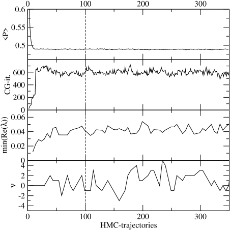
Figure 1: Equilibration signals for $\beta=5.2$, $a\,m=0.03$; from top to bottom: the plaquette mean, the number of CG iterations for the accept/reject step, the lower bound $\min(Re(\lambda))$ for the real part of the eigenvalues of the Dirac operator $D_{\textrm{\scriptsize{CI}}}(m)$, the topological charge $\nu$. The lower two rows’ values have been determined only for every 5th configuration.

As an example of the equilibration process we show in Fig. 1 some observables computed in the run-sequence for $\beta_{1}=5.2$ and $a\,m=0.03$. This run was started from a cold gauge configuration and one finds that the plaquette quickly approaches its equilibrium value. Another useful, more technical, observable is the number of CG iterations necessary in the accept/reject step. There equilibrium values are obtained somewhat later.

In Fig. 1 we also plot the development of the lower bound to the real parts of the eigenvalues of $D_{\textrm{\scriptsize{CI}}}(0.03)$. The value for every 5th configuration is shown. This quantity is a good indicator of the equilibration as it is most likely the largest time scale in the problem. At the same time it indicates the quality of the Dirac operator. Configurations, where the smallest eigenvalue becomes zero would lead to spurious zero modes. The amount of fluctuation of the observed lower bound also indicates the uncertainty width of the choice of the mass.

In the last row in Fig. 1 we show the topological charge $\nu$, again determined for every 5th configuration. The definition and determination is discussed in Sect. IV.1. Starting at a cold configuration initially locks the topological charge to the trivial sector. However, following the initial equilibration period, we find satisfactory fluctuation.

Altogether, based on such observations, we discarded the first 100 HMC trajectories before starting the analyzing measurements. The data are not sufficient to find reliable estimates for the autocorrelation length. Judging from the inspection of the fluctuation we estimate autocorrelation times of 10-20. Runs on the smaller lattice size had larger autocorrelation times LaMaOr05a . We analyzed every 5th configuration, determining hadron correlators and eigenvalues as discussed in Sect. IV.

All our runs were done with MPI parallelization, typically on 8 or 16 nodes on the Hitachi SR8000 (at LRZ Munich) or on 8 or 16 nodes of two Opteron 248 processors at 2.2 GhZ per processor. To get an estimate on timing, we note that for the $12^{3}\times 24$ lattice at $a\,m=0.05$ one trajectory takes $\sim 4$ hours on 8 nodes of the Hitachi; one trajectory at $a\,m=0.02$ takes $\sim 7$ hours on 16 of the double Opteron nodes.

IV What do we learn

The numbers that are presented here are affected by various limitations:

• We consider only two flavors of mass-degenerate quarks.

• The typical physical lattice in spatial direction is only up to 1.55 fm. We thus may expect to see finite volume effects.

• The statistics is limited; most of the runs discussed amount to typically 200 to 350 units of HMC time corresponding to 40 to 70 independent configurations.

• The smallest quark mass parameters correspond to a pion mass around 500 MeV, the smallest pion over rho mass ratio is 0.55.

• Only a small range of lattice spacing values between 0.11 fm and 0.13 fm is covered.

All these constraints are typical for first simulations with dynamical quarks, in particular in view of the computationally demanding properties of the Dirac operator. We therefore consider this study as the first but necessary step towards studies on larger and finer lattices with better statistics.

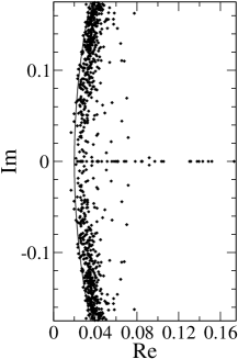
Figure 2: Plot of the 40 smallest eigenvalues of $D_{\textrm{\scriptsize{CI}}}(0.02)$ for a total of 21 configuration in equilibrium (run (a), lattice size $12^{3}\times 24$, $\beta_{1}=5.2$, $a\,m=0.02$).

IV.1 Eigenvalues and topology

Dirac operators obeying the GW condition in its simplest form have a characteristic eigenvalue spectrum: all eigenvalues are constrained to lie on a unit circle. The operator $D_{\textrm{\scriptsize{CI}}}$ is only an approximate GW operator and its eigenvalues are close to but not exactly on this so-called GW circle (radius 1, center at 1 in the complex plane). As a first test we studied the low-lying eigenvalues of $D_{\textrm{\scriptsize{CI}}}$ for some gauge configurations obtained with dynamical quarks.

Fig. 2 exhibits the accumulated eigenvalues for 21 configurations, where we determined the 40 smallest eigenvalues for each configuration. The curve indicates the eigenvalue circle for an exact GW operator for mass $a\,m=0.02$. The bulk of the eigenvalues closely follows the circular shape. A comparison of the spectra on smaller lattices with the quenched case has been presented in Ref. LaMaOr05a .

The complex eigenvalues come in complex conjugate pairs $\lambda_{i}$ and $\overline{\lambda}_{i}$ and always have vanishing chirality $\langle\psi_{i}|\gamma_{5}|\psi_{i}\rangle$. The real eigenvalues, which would be exact zero modes for exact GW operators, correspond to topological charges via the Atiyah-Singer index theorem AtSi71 ; HaLaNi98 . For the overlap Dirac operator only zero modes either all positive or all negative chirality have been observed. In our case we sometimes (in about 3% of the configurations) find zero modes with opposite chiralities as well.

We did compute the chiralities of the real (zero-)modes for the runs at $\beta=5.2$. The distribution is not symmetric but this is non-significant due to the relatively small sample. A symmetrized histogram is in good agreement with the Gaussian shape. In Fig. 3 we show the resulting histograms together with a Gaussian distribution with zero mean and the same second moment $\langle\nu^{2}\rangle$. As is well-known from experience with other Dirac operators, when evaluated over longer HMC-periods than the ones available to us, the tunneling frequency may show much longer correlation time AlBaDe98 ; AoBlCh04 .

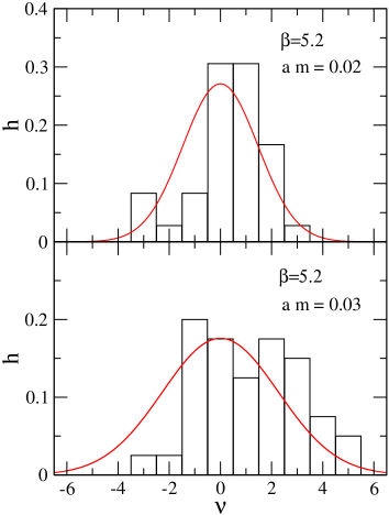
Figure 3: The distribution of the topological charge for the two runs at $\beta=5.2$ and $\,m=0.02$ and 0.03. We also show a fit to a Gaussian distribution function with the same $\langle\nu^{2}\rangle$.

Tunneling between different topological sectors appears to be a problem for HMC implementations of the overlap action; various intricate methods have been suggested to deal with it FoKaSz0405 ; EgFoKa05 ; CuKrFr05 ; CuKrLi05 ; DeSc05a ; DeSc05b . As can been seen in the lowest row of Fig. 1 we do not seem to have such a problem and observe frequent tunneling.

As mentioned, we determined the eigenvalues and thus the topological charge only for every 5th configuration. Comparing the number of changes of the topological sector we get (for the runs (a,b,d) and (e)) between 12 and 19 such changes along a HMC-time distance of 100, without obvious correlation to the run parameters. E.g., runs (d) and (e) have the same values of $\beta_{1}$ and $m$, but different lattice sizes. The width of the distribution of the smaller lattice is smaller, as expected, but the number of tunneling events comparable. These values are a lower bound for the actual number of tunneling events. In view of these we do not find the drastic dependence of the tunneling rate on the quark mass observed in simulations with the overlap action DeSc05b .

The topological susceptibility

$$\chi_{\textrm{\scriptsize{top}}}=\langle\nu^{2}\rangle/V$$ (13)

plays a central role in the Witten-Veneziano formula Wi79 ; Ve79 ; Ve80 . Due to the axial anomaly the quenched susceptibility (in the large $N_{c}$-limit) is related to the $\eta^{\prime}$-mass via

$$\chi_{\textrm{\scriptsize{top}}}^{quenched}=\frac{f_{\pi}^{2}\,m_{\eta^{\prime}}^{2}}{2N_{f}}\;.$$ (14)

(Here $f_{\pi}\approx 92\;\textrm{MeV}$ denotes the pion decay constant and $N_{f}$ the number of flavors, both defined in full QCD.) In quenched simulations values of $\chi_{\textrm{\scriptsize{top}}}\approx(190\ \textrm{MeV})^{4}$ have been found GaHoSc02 ; DePi04 ; DeGiPi05 . For the dynamical case the dependence of $\chi_{\textrm{\scriptsize{top}}}$ on $N_{f}$ and $m$ has been discussed recently, along with a consistent definition of the quantity GiRoTe02 ; Se02 ; GiRoTe04 ; Lu04 . Due to the anomalous Ward identity for the U(1) axial current the topological susceptibility for full QCD should vanish (in the chiral limit). As in formal continuum theory Cr77 ; LeSm92 the topological susceptibility (now for dynamical fermions) and the chiral condensate are related via

$$\chi_{\textrm{\scriptsize{top}}}^{dyn}=-\frac{m\,\Sigma}{N_{f}}+{\cal O}(m^{2})\;.$$ (15)

where $\Sigma$ denotes the condensate contribution per flavor degree of freedom.

The precision of our results for $\chi_{\textrm{\scriptsize{top}}}$ is too poor to verify the linear behavior in the quark mass. For the runs (a) and (b) of Table 1 we obtain in physical units the values

$$\chi_{\textrm{\scriptsize{top}}}^{dyn}(a) = (146(8)\;\textrm{MeV})^{4}\;,$$

$$\chi_{\textrm{\scriptsize{top}}}^{dyn}(b) = (166(8)\;\textrm{MeV})^{4}\;.$$ (16)

In these cases we do find, as expected, that our values are definitely smaller than the quenched ones.

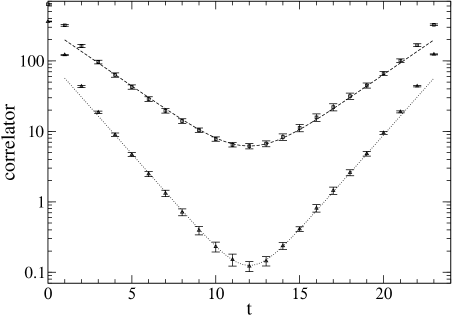
Figure 4: Correlation function for run (b), for the pseudoscalar (top) and the vector (bottom) meson. The curves give the results of fits to the $\cosh$-behavior as discussed in the text.

Table 2: Meson masses

#	$aM_{\pi}$	$aM_{\rho}$	$M_{\pi}/M_{\rho}$	$M_{\pi}$[MeV]	$M_{\rho}$[MeV]
a	0.292(10)	0.535(35)	0.55(5)	501(44)	918(109)
b	0.378(8)	0.619(30)	0.61(4)	597(42)	977(96)
c	0.326(18)	0.502(21)	0.65(6)	534(48)	823(62)
d	0.431(8)	0.626(18)	0.69(3)	657(16)	954(33)

IV.2 Meson masses

For the determination of the correlation function we used point quark sources and Jacobi-smeared sinks. Our definition and notation for the Jacobi smearing followed the quenched studies in BuGaGl05a ; GaHuLa05a . We used the narrow smearing distribution. Smearing the sink crucially improves the correlator signal quality and is almost as efficient as smearing source and sink.

The meson interpolating field were the usual ones:

$$\textrm{Pseudoscalar:}\quad P = \overline{d}\,\gamma_{5}\,u\;,$$ (17)

$$A_{4} = \overline{d}\,\gamma_{5}\gamma_{4}\,u\;,$$ (18)

$$\textrm{Vector:}\quad V_{k} = \overline{d}\,\gamma_{k}\,u\;,$$ (19)

where $u$ and $d$ denote the up- and down quark fields; $A_{4}$ is the temporal component of the axial vector, which also couples to the pion.

We computed the correlation functions

$$\langle P(\vec{p}=0,t)P(0)\rangle\;,$$ (20)

$$\langle A_{4}(\vec{p}=0,t)A_{4}(0)\rangle\;,$$ (21)

$$\langle V_{i}(\vec{p}=0,t)V_{i}(0)\rangle\;.$$ (22)

The result (see, e.g., Fig. 4) was then fitted to

$$C(t)=D(M)\,\left(\mathrm{e}^{-M\,t}\pm\mathrm{e}^{-M\,(T-t)}\right)\;.$$ (23)

The masses thus may be derived from the exponential decay and other low energy parameters from its coefficient.

We discuss here only results for the large lattice size $12^{3}\times 24$. There the fits were done in the range $(t_{a},\,t_{b})=(6,18)$. Table 2 summarizes our results for the masses. All error bars have been determined with the jack-knife method. We also checked that $\chi^{2}/d.o.f.$ for all the fits were $<1$. The results for the $\langle A_{4}A_{4}\rangle$ correlator were consistent with that for the $\langle PP\rangle$ correlation function, but with slightly larger statistical errors. In the table we therefore quote the pion mass obtained from the $\langle PP\rangle$ correlator.

IV.3 AWI mass and pion decay constant

The axial Ward identity (AWI) allows one to define the renormalized quark mass through the asymptotic behavior of the ratio

$$\frac{Z_{A}}{Z_{P}}\,\frac{\langle\,\partial_{t}A_{4}(\vec{p}=\vec{0},t)\,X(0)\,\rangle}{\langle\,P(\vec{p}=\vec{0},t)\,X(0)\,\rangle}=Z_{m}\,2\,m=2\,m^{(r)}\;,$$ (24)

where $X$ is any interpolator coupling to the pion and $Z_{A}$, $Z_{P}$ and $Z_{m}$ denote the renormalization factors relating the $\overline{\mbox{MS}}$-scheme at a scale of 2 GeV. These have been calculated for the quenched case at several values of the lattice spacing and came out close to 1 GaGoHu04 . We do not know the value for the dynamical case but for the mass values presented we expect it to be close to the quenched one. We therefore compute the ratio

$$\frac{\langle\,\partial_{t}A_{4}(\vec{p}=\vec{0},t)\,P(0)\,\rangle}{\langle\,P(\vec{p}=\vec{0},t)\,P(0)\,\rangle}\equiv 2\,m_{\textrm{\scriptsize{AWI}}}\;,$$ (25)

defining the so-called AWI-mass.

We measure

$$\langle A_{4}(\vec{p}=0,t)P(0)\rangle\;,$$ (26)

in order to construct

$$\langle\partial_{t}A_{4}(\vec{p}=0,t)P(0)\rangle\;.$$ (27)

Ratios involving the lattice derivative $\partial_{t}A_{4}$ depend on the way the derivative is taken. Numerical derivatives are always based on assumptions on the interpolating function. Usual simple 2- or 3-point formulas assume polynomials as interpolating functions. We can do better by utilizing the information on the expected $\sinh$-dependence. In fact, we may use this function for local 3-point $(t-1,\,t,\,t+1)$ interpolation and get the derivative at $t$ therefrom. We cannot use correlators like $\langle X(t)\,\partial_{t}A_{4}(0)\rangle$ since the source is fixed to the time slice $t=0$ and thus we cannot construct the lattice derivative there.

Eq. (25) assumes interpolating fields with point quark sources. The Jacobi-smearing of the quark sinks introduces a normalization factor relative to point sinks. The factors can be obtained from the asymptotic (large $t$) ratios of, e.g.,

$$c_{P}=\frac{\langle P(t)P\rangle}{\langle P_{s}(t)P\rangle}\;,\quad c_{A}=\frac{\langle A_{4}(t)P\rangle}{\langle A_{4,s}(t)P\rangle}\;,$$ (28)

where the index $s$ denotes the interpolator built from smeared sources. We find values of $c_{P}/c_{A}$ around 0.6 indicating that the smearing of the quarks affects the two operators differently, which may be understood from their different Dirac content and “wave function”. We did check that the results agree with that derived directly from correlators based on point-like quark sinks, only the error bars are slightly larger in the latter case. All numbers given refer to the normalization for operators built from point-like quark sources and sinks.

Taking this into account we find the AWI-mass from plateau values like that shown in Fig. 5. The final average was taken in the same interval as was used for the mass analysis and the error was again computed with the jack-knife method. The results are given in Table 3.

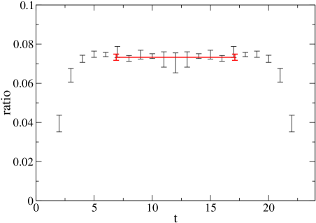
Figure 5: The ratio (25) for $\beta=5.2$, $a\,m=.03$. The plateau fit range is indicated.

In full, renormalized QCD the Gell-Mann–Oakes–Renner (GMOR) relation relates the pion and quark masses:

$$f_{\pi}^{2}\,M_{\pi}^{2}=-2\,m\,\Sigma\;.$$ (29)

Here two flavors of mass-degenerate quarks are assumed. The quark mass and the condensate (contribution per flavor d.o.f.) are renormalization scheme dependent and have to be given in, e.g., the $\overline{\mbox{MS}}$-scheme. Since the AWI-mass is proportional to the renormalized quark mass, this linear relationship may hold. Indeed, in lattice calculations surprisingly linear behavior has been found.

Table 3: Results for the AWI-mass in lattice units, and the AWI-mass, $M_{\pi}$ and the pion decay constant in units of the Sommer-parameter $r_{0}$ (which is usually assumed to be 0.5 fm).

#	$am_{\textrm{\scriptsize{AWI}}}$	$r_{0}^{2}M_{\pi}^{2}$	$r_{0}\,m_{{\textrm{\scriptsize{A}}}WI}$	$r_{0}\,f_{\pi}$
a	0.025(1)	1.62(28)	0.103(9)	0.237(44)
b	0.037(1)	2.29(33)	0.147(10)	0.321(45)
c	0.037(2)	1.84(33)	0.154(13)	0.314(44)
d	0.050(1)	2.78(14)	0.195(6)	0.281(26)

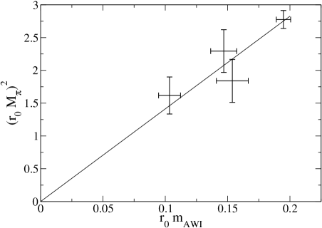
Figure 6: The pion mass squared vs the AWI-mass in units of the Sommer parameter $r_{0}$ for all 4 data sets (a–d). The fitted line corresponds to the lowest order chiral perturbation theory behavior, i.e., to the GMOR relation (29).

In Fig. 6 we plot our results for $M_{\pi}^{2}$ and $m_{\textrm{\scriptsize{AWI}}}$ for all four runs. Within the errors the results are compatible with the expected linear dependence. Neglecting the renormalization factors and taking the experimental value 92 MeV for the pion decay constant the slope, via (29) corresponds to a value for the condensate of $\Sigma=(288(8)\;\textrm{MeV})^{3}$. The errors are purely statistical, from the fit to the straight line, neglecting possible higher order chiral perturbation theory contributions.

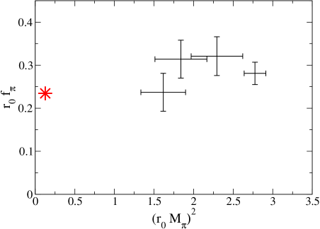
Figure 7: $f_{\pi}$ vs pion mass squared in units of the Sommer parameter $r_{0}$ for all 4 data sets (a–d). The $\ast$ denotes the experimental value.

We can now go ahead and obtain the pion decay constant $f_{\pi}$. It is related to the coefficient of the $\langle A_{4}A_{4}\rangle$ correlator with point source and sink and may be extracted through its asymptotic (large $t$) behavior:

$$Z_{A}^{2}\langle A_{4}(\vec{p}=\vec{0},t)A_{4}(0)\rangle\stackrel{{\scriptstyle\textrm{\scriptsize large $t$}}}{{\longrightarrow}}M_{\pi}f_{\pi}^{2}e^{-M_{\pi}t}\;.$$ (30)

Again we assume $Z_{A}\approx 1$; in Fig. 7 we show the results, which are compatible with the experimental values. For this measurement we actually used the point - point correlation function. Table 3 summarizes our results in units of the Sommer parameter.

V Summary/Conclusion

We have implemented the Chirally Improved Dirac operator, obeying the GW condition to a good approximation, in a simulation with two species of mass-degenerate light quarks. In our simulations on $12^{3}\times 24$-lattices the lattice spacing was as small as 0.115 fm. The quark masses reached so far correspond to a $M_{\pi}/M_{\rho}$ ratio of 0.55.

We consider this as a first step towards the final goal to approach realistic quark masses. Nice features of the $D_{\textrm{\scriptsize{CI}}}$, which were observed in quenched simulations, like the spectrum following the GW circle, appear to hold in the dynamical case as well. The good consistency of the results with experimental numbers seems to indicate, that the renormalization factors are close to 1 (as they have been found in the quenched case). We also find no evidence for spurious zero modes and we therefore do not expect serious problems to go down further in the quark mass.

The results are encouraging and demonstrate that the CI operator is well suited for dynamical fermion simulations.

- (1) P. H. Ginsparg and K. G. Wilson, Phys. Rev. D 25, 2649 (1982).
- (2) R. Narayanan and H. Neuberger, Phys. Lett. B 302, 62 (1993); Nucl. Phys. B443, 305 (1995).
- (3) H. Neuberger, Phys. Lett. B 417, 141 (1998); Phys. Lett. B 427, 353 (1998).
- (4) Z. Fodor, S. D. Katz, and K. K. Szabo, JHEP 0408, 003 (2004); Nucl. Phys. Proc. Suppl. 140, 704 (2005).
- (5) G. I. Egri, Z. Fodor, S. D. Katz, and K. Szabo, Topology with dynamical overlap fermions, 2005 hep-lat/0510117
- (6) N. Cundy, S. Krieg, A. Frommer, T. Lippert, and K. Schilling, Nucl. Phys. Proc. Suppl. 140, 841 (2005).
- (7) N. Cundy, S. Krieg, and T. Lippert, Proc. Sci. LAT2005, 107 (2005).
- (8) T. DeGrand and S. Schaefer, Phys. Rev. D 71, 034507 (2005).
- (9) T. DeGrand and S. Schaefer, Phys. Rev. D 72, 054503 (2005).
- (10) D. B. Kaplan, Phys. Lett. B 288, 342 (1992).
- (11) V. Furman and Y. Shamir, Nucl. Phys. B439, 54 (1995).
- (12) Y. Aoki et al., Lattice QCD with two dynamical flavors of domain wall quarks, 2004, hep-lat/0411006.
- (13) D. J. Antonio et al., Proc. Sci. LAT2005, 080 (2005).
- (14) P. Hasenfratz and F. Niedermayer, Nucl. Phys. B414, 785 (1994).
- (15) A. Hasenfratz, P. Hasenfratz, and F. Niedermayer, Simulating full QCD with the fixed point action, 2005, hep-lat/0506024.
- (16) C. Gattringer, Phys. Rev. D 63, 114501 (2001).
- (17) C. Gattringer, I. Hip, and C. B. Lang, Nucl. Phys. B597, 451 (2001).
- (18) C. Gattringer et al., Nucl. Phys. B677, 3 (2004).
- (19) C. B. Lang, P. Majumdar, and W. Ortner, Proc. Sci. LAT2005, 124 (2005).
- (20) C. B. Lang, P. Majumdar, and W. Ortner, Proc. Sci. LAT2005, 131 (2005).
- (21) A. Hasenfratz and F. Knechtli, Phys. Rev. D 64, 034504 (2001).
- (22) C. Morningstar and M. Peardon, Phys.Rev. D 69, 054501 (2004).
- (23) M. Lüscher and P. Weisz, Commun. Math. Phys. 97, 59 (1985); Err. ibid. 98, 433 (1985).
- (24) M. Alford, W. Dimm, G. P. Lepage, G. Hockney, and P. B. Mackenzie, Phys. Lett. B 361, 87 (1995).
- (25) S. Duane, A. D. Kennedy, B. J. Pendleton, and D. Roweth, Phys. Lett. B 195, 216 (1987).
- (26) S. Gottlieb, W. Liu, D. Toussaint, R. L. Renken, and R. L. Sugar, Phys. Rev. D 35, 2531 (1987).
- (27) R. C. Brower, T. Ivanenko, A. R. Levi, and K. N. Orginos, Nucl. Phys. B484, 353 (1997).
- (28) R. Sommer, Nucl. Phys. B411, 839 (1994).
- (29) M. Atiyah and I. M. Singer, Ann. Math. 93, 139 (1971).
- (30) P. Hasenfratz, V. Laliena, and F. Niedermayer, Phys. Lett. B 427, 125 (1998).
- (31) B. Alles et al., Phys.Rev. D 58, 071503 (1998).
- (32) E. Witten, Nucl. Phys. B156, 269 (1979).
- (33) G. Veneziano, Nucl. Phys. B159, 213 (1979).
- (34) G. Veneziano, Phys. Lett. B 95, 90 (1980).
- (35) C. Gattringer, R. Hoffmann, and S. Schaefer, Phys. Lett. B 535, 358 (2002).
- (36) L. D. Debbio and C. Pica, JHEP 02, 003 (2004).
- (37) L. D. Debbio, L. Giusti, and C. Pica, Phys.Rev.Lett. 94, 032003 (2005).
- (38) L. Giusti, G. C. Rossi, M. Testa, and G. Veneziano, Nucl. Phys. B628, 234 (2002).
- (39) E. Seiler, Phys. Lett. B 525, 355 (2002).
- (40) L. Giusti, G. Rossi, and M. Testa, Phys. Lett. B 587, 157 (2004).
- (41) M. Lüscher, Phys.Lett. B 593, 296 (2004).
- (42) R. J. Crewther, Phys. Lett. B 70, 349 (1977).
- (43) H. Leutwyler and A. Smilga, Phys. Rev. D 46, 5607 (1992).
- (44) T. Burch et al., Nucl. Phys. Proc. Suppl. 140, 284 (2005).
- (45) C. Gattringer, P. Huber, and C. B. Lang, Phys. Rev. D 72, 094510 (2005).
- (46) C. Gattringer, M. Göckeler, P. Huber, and C. B. Lang, Nucl. Phys. B694, 170 (2004).