Light meson masses and decay constants in 2+1 flavour domain wall QCD

Abstract:

We present results for light meson masses and psedoscalar meson decay constants in 2+1 flavour domain wall QCD with the DBW2 and Iwasaki gauge actions, using lattices with linear sizes in the range 1.6 to 2.2fm and $u$ and $d$ quark masses as low as one quarter of the strange quark mass. All data were generated on the QCDOC machines at the University of Edinburgh and Brookhaven National Laboratory. Despite large residual masses and a limited number of sea quark mass values with which to perform chiral extrapolations, our results agree with experiment and scale within errors.

PoS(LAT2005)080

1 INTRODUCTION

The application of the RHMC algorithm [1] to lattice QCD with Ginsparg-Wilson quarks together with the computational power of QCDOC has resulted in the ability to generate, and perform measurements on, dynamical 2+1 flavour configurations for the first time. However, before embarking on a large-scale and (potentially) computationally costly production run, it is necessary to explore the available parameter space with (several) smaller and, therefore, computationally cheaper initial trials. This work focuses on the recent ensembles generated on the QCDOC machines for exactly this purpose.

2 SIMULATION PARAMETERS

The analysis was carried out on 2+1 flavour domain wall fermion configurations generated on the QCDOC machines. The standard domain wall Dirac operator [2] and Pauli-Villars field with the action introduced in [3] was used. The gauge action was defined by

$$S_{G}[U]=-\frac{\beta}{3}\left[(1-8\,c_{1})\sum_{x;\mu<\nu}P[U]_{x,\mu\nu}+c_{1}\sum_{x;\mu\neq\nu}R[U]_{x,\mu\nu}\right]$$ (1)

where $P[U]_{x,\mu\nu}$ and $R[U]_{x,\mu\nu}$ represent the real part of the trace of the path ordered product of links around the $1\times 1$ plaquette and $1\times 2$ rectangle, respectively, in the $\mu,\nu$ plane at the point $x$, and $\beta\equiv 6/g^{2}$ with $g$ the bare coupling constant. For the DBW2 gauge action [4, 5], the coefficient $c_{1}$ was chosen to be $-1.4069$, whereas for Iwasaki [6, 7] $c_{1}=-0.331$. In the DBW2 case the ensembles have three different $\beta$ values: 0.72, 0.764 and 0.78, while for the Iwasaki case they have two: 2.13 and 2.2. All ensembles were generated using the RHMC algorithm [1] with a trajectory length of 0.5, volume of $16^{3}$x32, fifth dimension length of 8, and a domain wall height of 1.8. Two different ensembles were generated at each $\beta$ value, one with a light isodoublet with mass $m_{ud}=\frac{1}{2}m_{s}$ and one where the light sea quark masses are both equal to our rough estimate of the strange quark mass, $m_{s}$. An additional DBW2 ensemble with a light isodoublet mass $m_{ud}=\frac{1}{4}m_{s}$ at $\beta$=0.72 was generated. The number of trajectories in each ensemble and the number of configurations used in the analysis are shown in table 1. The ensembles had $am_{ud}$ = 0.01, 0.02 or 0.04 and $am_{s}$ = 0.04.

Measurements were made with up to four valence quark masses in the range 0.01 to 0.04 on each ensemble and, on some of the ensembles, correlators were measured with sources on multiple time planes to improve our statistics. Several types of smearing were used, in particular, point sources, wall sources, and hydrogen-like wavefunction smearing where one or two of the quark propagators in a meson correlator were smeared at the source. In general, simultaneous fits to local and smeared correlators were performed throughout. This analysis aggregates to more than thirty thousand trajectories and more than one hundred and twenty thousand measurements.

The integrated auto-correlation time for the pseudoscalar meson correlator was calculated on several of these ensembles and found to be of order 100 trajectories. The correlators were oversampled and averaged into bins of size between five and ten depending on whether the separation between measurements was five or ten trajectories. Our observed errors stabilised with bins of this size in good agreement with the calculated integrated auto-correlation time. A full correlated analysis was then performed with the binned data as input.

Action	$\beta$	$\frac{m_{ud}}{m_{s}}$	$am_{ud}$	$N_{traj}$	$N_{meas}$	$am_{\rm res}$
DBW2	0.72	1.0	0.04	3395	475
DBW2	0.72	0.5	0.02	6000	1000	0.0106(1)
DBW2	0.72	0.25	0.01	2340	269
DBW2	0.764	1.0	0.04	1615	150
DBW2	0.764	0.5	0.02	1800	88	0.00546(7)
DBW2	0.78	1.0	0.04	1620	113
DBW2	0.78	0.5	0.02	1505	202	0.00437(6)
Iwasaki	2.13	1.0	0.04	2380	139
Iwasaki	2.13	0.5	0.02	2450	146	0.0104(2)
Iwasaki	2.2	1.0	0.04	4565	713
Iwasaki	2.2	0.5	0.02	3175	435	0.0065(1)

Table 1: RHMC 2+1 flavour datasets and the value of the residual mass in the chiral limit.

3 RESULTS

3.1 The Residual Mass

The residual mass is a measure of the violation of chiral symmetry [2]. In our ensembles the length of the fifth dimension is relatively short, hence there is a significant left-right coupling between the quark fields on opposite walls. The residual mass was calculated from the ratio of the point-split pseudoscalar density $J_{5}$ at the middle of the fifth dimension to the pseudoscalar density P built from the fields on the walls [2]

$$am_{\rm res}=\frac{\Sigma_{\vec{x},\vec{y}}\langle J_{5}(\vec{y},t)P(\vec{x},0)\rangle}{\Sigma_{\vec{x},\vec{y}}\langle P(\vec{y},t)P(\vec{x},0)\rangle}.$$ (2)

A good signal for the value of $am_{\rm res}$ was observed, as can be seen in figure 1 (left).

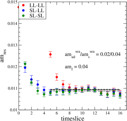
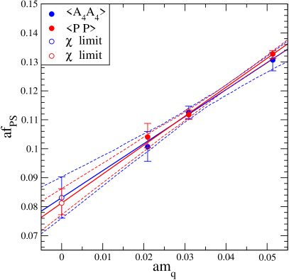
Figure 1: LEFT: Residual mass for $\beta$ = 2.13 ensemble with $m_{ud}=\frac{1}{2}m_{s}$. Different colours correspond to whether zero, one or two quark propagators are smeared at the source. RIGHT: Pseudoscalar meson decay constant using two different methods versus quark mass for the DBW2 $\beta$=0.72 ensembles.

Chiral extrapolations were performed by defining the quark mass

$$am_{q}\equiv a(m_{f}+m_{\rm res}(m_{f})),$$ (3)

where $am_{f}$ is the valence quark mass and $m_{\rm res}(m_{f})$ is the residual mass measured using quark propagators with that quark mass, and taking $am_{q}\rightarrow 0$ using only the points where the valence quark mass is equal to the $u$ and $d$ quark masses in the sea. Other than in the DBW2 $\beta$=0.72 case, where a linear fit to three points was performed, straight lines were drawn through the two available points. The values of the residual mass obtained in the chiral limit are shown in table 1. These values correspond to a residual mass of $\sim$5-30 MeV.

3.2 Light hadron masses

Pseudoscalar and vector meson masses are extracted by performing simultaneous double cosh fits to extract both the ground and first excited states.

Chiral extrapolations were performed in an analogous way to the residual mass by extrapolating the results to $m_{q}$ = 0. In the case of the pseudoscalar mass this takes the form

$$(am_{PS})^{2}=B(am_{q}^{val=sea})+A.$$ (4)

Given the low statistics, an acceptable slight deviation of $A$ from zero, typically less than 2$\sigma$, is observed. The lattice spacing was obtained from $m_{\rho}$ in the chiral limit by performing a linear chiral extrapolation of the vector meson mass

$$am_{V}=C(am_{q}^{val=sea})+D.$$ (5)

This, together with the physical kaon mass and substituting $am_{q}^{val=sea}\rightarrow am_{q_{1}}+am_{q_{2}}$ in eq.( 4), allowed the evaluation of the strange quark mass by setting $am_{q_{1}}=am_{ud}=0$ and $am_{q_{2}}=am_{s}$.

3.3 Pseudoscalar meson decay constants

The pseudoscalar meson decay constant defined by

$$af_{PS}=\frac{Z_{A}\langle 0|A_{4}|P\rangle}{am_{PS}}$$ (6)

was calculated in two ways. In the first method $Z_{A}$ was obtained from the axial Ward-Takahashi identity

$$Z_{A}\langle\partial_{\mu}A_{\mu}\mathcal{O}\rangle=2(am_{q}+am_{\rm res})\langle P\mathcal{O}\rangle$$ (7)

which can be expressed in terms of the pseudoscalar meson correlator, $C_{PP}$, and the pseudoscalar meson axial correlator, $C_{PA_{4}}$. $\langle 0|A_{4}|P\rangle$ cancels when $Z_{A}$ is substituted in eq.(6) and hence only $C_{PP}$ and the value of the residual mass are required in order to evaluate $f_{PS}$

$$af_{PS}=\frac{2(am_{f}+am_{\rm res})\langle 0|P|P\rangle}{(am_{PS})^{2}}.$$ (8)

The red symbols in figure 1 (right) show the chiral extrapolation of $f_{PS}$ for the DBW2 $\beta$=0.72 ensembles.

In the second method, we calculated the value of $Z_{A}$ explicitly from a ratio designed to remove $\mathcal{O}$(a) and suppress $\mathcal{O}$($a^{2}$) lattice artifacts [8].

$$Z_{A}=\frac{C(t+\frac{1}{2})+C(t-\frac{1}{2})}{4L(t)}+\frac{C(t+\frac{1}{2})}{(L(t)+L(t+1))}$$ (9)

where $C(t)$ and $L(t)$ are the correlators of the pseudoscalar density with the partially conserved and local axial currents respectively. A simultaneous fit to both point-point and wall/smeared-point correlators is used to extract this ratio. The axial-axial correlator was then used in combination with the value of $Z_{A}$ to calculate the pseudoscalar meson decay constant. The chiral extrapolation of $f_{PS}$ using this method is shown by the blue symbols in figure 1 (right). We see good agreement between both methods.

Using the lattice spacing and the strange quark mass calculated from the vector meson and pseudoscalar meson chiral extrapolations, we are able to calculate $f_{K}$ and extract the ratio $\frac{f_{K}}{f_{\pi}}$.

3.4 Scaling

The ensembles generated for this analysis with several different lattice spacings and two different gauge actions have $\mathcal{O}$($a^{2}$) discretisation errors. Figure 2 (left) shows the ratio $\frac{f_{K}}{f_{\pi}}$ plotted against lattice spacing squared. The different colour symbols correspond to the different gauge actions, Iwasaki in blue and DBW2 in red. We have set the lattice spacing in two different ways. The closed symbols correspond to setting the lattice spacing from the $\rho$ meson mass, while the open symbols are from setting the lattice spacing from $f_{\pi}$. Note that the errors are still quite large. The furthest two points to the right are the DBW2 $\beta$=0.72 points where we have been able to perform a chiral fit compared to drawing straight lines through the points so their errors are better estimated. Even with the large and crude error estimate for the other results, it may be concluded that there is an indication of scaling and, if anything, scaling may slightly better for the Iwasaki gauge action than for DBW2. Figure 2 (right) shows a similar plot to figure 2 (left), for $\frac{m_{K*}}{m_{\rho}}$ and similar behaviour is seen.

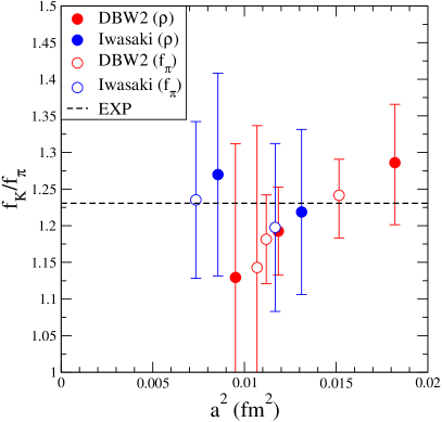
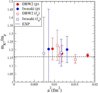
Figure 2: Scaling behaviour of LEFT: $\frac{f_{K}}{f_{\pi}}$ and RIGHT: $\frac{m_{K^{*}}}{m_{\rho}}$ for all ensembles. Different colours correspond to different gauge actions. Open and closed symbols correspond to setting the lattice spacing from $f_{\pi}$ or $m_{\rho}$ in the chiral limit respectively.

4 SUMMARY

Several ensembles have been generated on the QCDOC machines using the domain wall fermion formulation with two different gauge actions, several $\beta$ values and multiple sea quark masses. These ensembles have a relatively small volume and limited statistics as they were primarily generated to search parameter space for a larger production run. A fifth dimension size of eight produces a residual mass larger than would be acceptable for such a production run. Even with these drawbacks it is still possible to calculate the light hadron spectrum and pseudoscalar decay constants obtaining results which are consistent with experiment and scale within large errors. At present we are running an ensemble with a larger volume of $24^{3}$x$64$ and a fifth dimension size of 16 using the Iwasaki gauge action at $\beta=2.13$.

5 ACKNOWLEDGEMENTS

We thank Sam Li and Meifeng Lin for help generating the datasets used in this work. We thank Dong Chen, Norman Christ, Saul Cohen, Calin Cristian, Zhihua Dong, Alan Gara, Andrew Jackson, Chulwoo Jung, Changhoan Kim, Ludmila Levkova, Xiaodong Liao, Guofeng Liu, Robert Mawhinney, Shigemi Ohta, Konstantin Petrov and Tilo Wettig for developing with us the QCDOC machine and its software. This development and the resulting computer equipment used in this calculation were funded by the U.S. DOE grant DE-FG02-92ER40699, PPARC JIF grant PPA/J/S/1998/00756 and by RIKEN. This work was supported by PPARC grant PPA/G/O/2002/00465.

References

- [1] M. A. Clark, A. D. Kennedy and Z. Sroczynski, Exact 2+1 flavour RHMC simulations, hep-lat/0409133.
- [2] V. Furman and Y. Shamir, Axial symmetries in lattice QCD with Kaplan fermions, Nucl. Phys. B439 (1995) 54–78 [hep-lat/9405004].
- [3] P. M. Vranas, Chiral symmetry restoration in the Schwinger model with domain wall fermions, Phys. Rev. D57 (1998) 1415–1432 [hep-lat/9705023].
- [4] T. Takaishi, Heavy quark potential and effective actions on blocked configurations, Phys. Rev. D54 (1996) 1050–1053.
- [5] QCD-TARO Collaboration, P. de Forcrand et. al., Renormalization group flow of SU(3) lattice gauge theory: Numerical studies in a two coupling space, Nucl. Phys. B577 (2000) 263–278 [hep-lat/9911033].
- [6] Y. Iwasaki, Renormalization group analysis of lattice theories and improved lattice action. 2. four-dimensional nonabelian SU(N) gauge model, . UTHEP-118.
- [7] Y. Iwasaki and T. Yoshie, Renormalization group improved action for SU(3) lattice gauge theory and the string tension, Phys. Lett. B143 (1984) 449.
- [8] T. Blum et. al., Quenched lattice QCD with domain wall fermions and the chiral limit, Phys. Rev. D69 (2004) 074502 [hep-lat/0007038].