$B\rightarrow D^{*}l\nu$ and $B\rightarrow Dl\nu$ form factors in staggered chiral perturbation theory

Abstract

We calculate the $B\to D$ and $B\to D^{*}$ form factors at zero recoil in Staggered Chiral Perturbation Theory. We consider heavy-light mesons in which only the light ($u$, $d$, or $s$) quark is staggered; current lattice simulations generally use a highly improved action such as the Fermilab or NRQCD action for the heavy ($b$ or $c$) quark. We work to lowest nontrivial order in the heavy quark expansion and to one-loop in the chiral expansion. We present results for a partially quenched theory with three sea quarks in which there are no mass degeneracies (the “1+1+1” theory) and for a partially quenched theory in which the $u$ and $d$ sea quark masses are equal (the “2+1” theory). We also present results for full (2+1) QCD, along with a numerical estimate of the size of staggered discretization errors. Finally, we calculate the finite volume corrections to the form factors and estimate their numerical size in current lattice simulations.

I Introduction

The CKM matrix element $|V_{cb}\,|$, which places an important constraint on the apex of the CKM unitarity triangle through the ratio $|V_{ub}/V_{cb}\,|$, can be determined from experimental measurements of exclusive semileptonic $B$-meson decays combined with theoretical input. Because experiments measure the product $({\cal F}(1)\cdot|V_{cb}\,|)^{2}$, where ${\cal F}(1)$ is the $B\to D$ or $B\to D^{*}$ hadronic form factor at zero recoil, the precision of $|V_{cb}\,|$ is limited by the theoretical uncertainty in ${\cal F}(1)$. Although, in principle, both form factors can be calculated nonperturbatively using lattice QCD, in practice, direct calculations of the $B\to D$ and $B\to D^{*}$ hadronic matrix elements are plagued by large statistical and systematic errors. Hashimoto et al. therefore proposed a method for calculating ${\cal F}(1)$ on the lattice using double ratios of matrix elements in which most of the statistical and systematic errors cancel Hashimoto et al. (2000, 2002). This method provides the key theoretical ingredient necessary to allow a precise lattice determination of the $B\to D$ or $B\to D^{*}$ form factors, and hence a precise determination of $|V_{cb}\,|$.

Recently ${\cal F}_{B\to D}$ was calculated using 2+1 flavors of dynamical staggered quarks Okamoto et al. (2005), and the analogous calculation of ${\cal F}_{B\to D^{*}}$ will be done in the near future. Because staggered quarks are computationally cheaper than other standard fermion discretizations, staggered simulations offer the lightest dynamical quark masses currently available Kennedy (2005). This result therefore has a smaller systematic error associated with chiral extrapolation than previous quenched results Hashimoto et al. (2002). It is known, however, that the ${\cal O}(a^{2})$ discretization errors associated with staggered fermions are numerically significant in current lattice simulations and must also be accounted for in the chiral and continuum extrapolation of staggered lattice data Aubin et al. (2004). This procedure is well-established in the light meson sector: use of staggered chiral perturbation theory Lee and Sharpe (1999); Aubin and Bernard (2003a, b); Sharpe and Van de Water (2005) functional forms for extrapolation of staggered lattice data has allowed precise determinations of light meson masses, meson decay constants, and even quark masses Aubin et al. (2004). Staggered chiral perturbation theory was recently extended to heavy-light mesons (in which only the light quark is staggered) by Aubin and Bernard Aubin and Bernard (2005), and has been successfully used in the extrapolation of the $D$-meson decay constant Aubin et al. (2005).

In this paper we use heavy-light staggered chiral perturbation theory to calculate the $B\to D$ and $B\to D^{*}$ form factors at zero recoil. The resulting functional forms can then be used to extrapolate staggered lattice data to the continuum and to the physical pion mass. Accounting for staggered discretization errors in this way is essential for a precise lattice determination of these form factors, and consequently of $|V_{cb}\,|$.

This paper is organized as follows. We review staggered chiral perturbation theory for heavy-light mesons in Section II. We then calculate the $B\to D$ and $B\to D^{*}$ form factors at zero recoil for a 1+1+1 PQ theory, a 2+1 PQ theory and full (2+1) QCD in Section III. Next, in Section IV, we plot the $B\to D$ and $B\to D^{*}$ form factors using reasonable values for the quark masses and lattice spacing both with and without the taste-symmetry breaking contributions. The dramatic change in the shape of the $B\to D^{*}$ form factor illustrates the necessity of accounting for taste-breaking in the continuum and chiral extrapolation of staggered lattice data. In Section V we use the method of Ref. Arndt and Lin (2004) to calculate the finite volume corrections to the $B\to D$ and $B\to D^{*}$ form factors. We then estimate the numerical size of these finite volume corrections in current lattice simulations; we find them to be very small – only one part in $10^{4}$. In Section VI we conclude. The Appendix contains additional formulae necessary to understand our form factor results. It follows the conventions of Ref. Aubin and Bernard (2003b).

II Staggered $\chi$PT with Heavy-Light Mesons

In this section we review staggered chiral perturbation theory (S$\chi$PT) for heavy-light mesons, which was developed in Ref. Aubin and Bernard (2005).

We first construct the portion of the heavy meson chiral Lagrangian that only contains light quark fields. We consider a partially quenched theory with $n$ flavors of staggered light quarks. The detailed construction of the leading-order effective staggered chiral Lagrangian is given in Ref. Aubin and Bernard (2003a); we simply present the results that are necessary for the calculation of the $B\to D$ and $B\to D^{*}$ form factors.

We assume that spontaneous symmetry breaking of the $SU(4n)$ chiral symmetry by the vacuum,

$$SU(4n)_{L}\times SU(4n)_{R}\rightarrow SU(4n)_{V}\,,$$ (1)

leads to $16n^{2}-1$ pseudo-Goldstone bosons, which we will generically call pions, that can be collected into an $SU(4n)$ matrix:

$$\Sigma=\exp(i\Phi/f)\,.$$ (2)

The matrix, $\Phi$, which contains the pion fields, is traceless with $4\times 4$ submatrices:

$$\Phi = \left(\begin{array}[]{cccc}U&\pi^{+}&K^{+}&\cdots\\ \pi^{-}&D&K^{0}&\cdots\\ K^{-}&\bar{K^{0}}&S&\cdots\\ \vdots&\vdots&\vdots&\ddots\end{array}\right),$$ (7)

$$U = \sum_{\Xi=1}^{16}U_{\Xi}T_{\Xi}\,,\;\;\textrm{etc.}$$ (8)

where the $SU(4)$ generators,

$$T_{\Xi}=\{\xi_{5},i\xi_{\mu 5},i\xi_{\mu\nu},\xi_{\mu},\xi_{I}\}\,,$$ (9)

are Euclidean gamma matrices and $\xi_{I}$ is the $4\times 4$ identity matrix. The leading order pion decay constant, $f$, is approximately $131\mathop{\rm MeV}\nolimits$. Like the pion matrix, the quark mass matrix is also $4n\times 4n$, but it has trivial taste structure:

$${\cal M}=\left(\begin{array}[]{cccc}m_{u}I&0&0&\cdots\\ 0&m_{d}I&0&\cdots\\ 0&0&m_{s}I&\cdots\\ \vdots&\vdots&\vdots&\ddots\end{array}\right)\,.$$ (14)

Under chiral symmetry transformations,

$$\Sigma\rightarrow L\Sigma R^{\dagger},$$ (15)

$${\cal M}\rightarrow L{\cal M}R^{\dagger},$$ (16)

$$L\in SU(4n)_{L},\;\;\;R\in SU(4n)_{R}.$$ (17)

The standard S$\chi$PT power-counting scheme is:

$$p_{\pi}^{2}/\Lambda_{\chi}^{2}\approx m_{q}/\Lambda_{\textrm{QCD}}\approx a^{2}\Lambda_{\textrm{QCD}}^{2}\,,$$ (18)

so the lowest-order, ${\cal O}(p_{\pi}^{2},m_{q},a^{2})$, staggered chiral Lagrangian is

$${\cal L}_{\textrm{S$\chi$PT}}^{\textrm{LO}} = \frac{f^{2}}{8}\textrm{Str}\big{[}\partial_{\mu}\Sigma\partial^{\mu}\Sigma\big{]}+\frac{f^{2}\mu}{4}\textrm{Str}\big{[}{\cal M}^{{\dagger}}\Sigma+\Sigma^{{\dagger}}{\cal M}\big{]}-\frac{2m^{2}_{0}}{3}\big{(}U_{I}+D_{I}+S_{I}\big{)}^{2}-a^{2}{\cal V}.$$

The staggered potential, ${\cal V}$, splits the tree-level pion masses into five degenerate groups,

$$\left(m_{\pi}^{2}\right)_{\rm LO}=\mu(m_{i}+m_{j})+a^{2}\Delta_{\Xi}\,,$$ (20)

according to their $SO(4)$-taste irrep, $\Xi=I,P,V,A,T$. It also leads to hairpin (quark-disconnected) propagators with multiple poles for flavor-neutral, taste $V$ and $A$ pions.

We now construct the remaining terms in the heavy meson chiral Lagrangian. Ref. Aubin and Bernard (2005) showed that, at ${\cal O}(a^{2})$, mixed four-fermion operators with both heavy and light quarks cannot break taste-symmetry. Because all taste-violation in the Symanzik action comes strictly from the light quark sector, discretization errors caused by mixed four-fermion operators can be categorized as “heavy-quark errors” and estimated using standard methods Kronfeld (2000, 2004). Thus the form of the heavy meson portion of the chiral Lagrangian is identical to that in the continuum, with the exception that the light quark index can run over both flavor and taste.

Heavy meson chiral perturbation theory (HM$\chi$PT) was first formulated in Refs. Burdman and Donoghue (1992); Wise (1992) and generalized to partially quenched QCD in Ref. Sharpe and Zhang (1996). Heavy quark spin symmetry allows the pseudoscalar and vector mesons to be combined into a single field which annihilates a heavy-light meson:

$$H_{a}=\frac{1+\not\!v}{2}[\gamma^{\mu}B^{*}_{\mu a}+i\gamma_{5}B_{a}],$$ (21)

where $v$ is the meson’s velocity and $a$ labels the flavor and taste of the light quark within the meson. Note that, although we use the letter $B$, the heavy-light meson can be either a $B$, in which the heavy quark is a $b$, or a $D$, in which the heavy quark is a $c$. We also define the conjugate field, $\overline{H}_{a}\equiv\gamma_{0}H_{a}^{\dagger}\gamma_{0}$, which creates a heavy-light meson.

Under heavy-quark spin symmetry,

$$H\rightarrow SH,\;\;\;\overline{H}\rightarrow\overline{H}S^{\dagger}$$ (22)

$$S\in SU(2),$$ (23)

while under chiral symmetry,

$$H\rightarrow HU^{\dagger},\;\;\;\overline{H}\rightarrow U\overline{H}$$ (24)

$$U\in SU(4n).$$ (25)

Interaction terms between heavy-light and pion fields are constructed using $\sigma=\sqrt{\Sigma}=\textrm{exp}[i\Phi/2f]$, which is invariant under heavy-quark spin symmetry but transforms under chiral symmetry as

$$\sigma\rightarrow L\sigma U^{\dagger}=U\sigma R^{\dagger},\;\;\;\sigma^{\dagger}\rightarrow R\sigma^{\dagger}U^{\dagger}=U\sigma^{\dagger}L^{\dagger}.$$ (26)

Heavy meson chiral perturbation theory is a joint expansion in the inverse of the heavy quark mass, $1/m_{Q}$, and in the residual momentum of the heavy-light meson, $k$. Thus the leading order heavy meson Lagrangian is of ${\cal O}(k)$:

$${\cal L}^{\textrm{LO}}_{\textrm{HM$\chi$PT}} = -i\textrm{tr}_{D}\big{[}\overline{H}_{a}v^{\mu}\big{(}\delta_{ab}\partial_{\mu}+iV^{ba}_{\mu}\big{)}H_{b}\big{]}+g_{\pi}\textrm{tr}_{D}\big{(}\overline{H}_{a}H_{b}\gamma^{\nu}\gamma_{5}A^{ba}_{\nu}\big{)},$$ (27)

where $V_{\mu}\equiv\frac{i}{2}\big{[}\sigma^{\dagger}\partial_{\mu}\sigma+\sigma\partial_{\mu}\sigma^{\dagger}\big{]}$, $A_{\mu}\equiv\frac{i}{2}\big{[}\sigma^{\dagger}\partial_{\mu}\sigma-\sigma\partial_{\mu}\sigma^{\dagger}\big{]}$ and $\textrm{tr}_{D}$ indicates a trace over Dirac spin indices. Combining this with the purely pionic terms, the total chiral Lagrangian for heavy-light mesons in which the light quark is staggered is

$${\cal L}^{\textrm{LO}}={\cal L}_{\textrm{HM$\chi$PT}}^{\textrm{LO}}+{\cal L}_{\textrm{S$\chi$PT}}^{\textrm{LO}}.$$ (28)

III Chiral Corrections to $B\to D$ and $B\to D^{*}$ at Zero Recoil

The hadronic matrix elements for $B\to D^{(*)}$ depend upon six independent form factors:

$$\langle D(v^{\prime})|\overline{c}\gamma^{\mu}b|\overline{B}(v)\rangle = h_{+}(w)(v+v^{\prime})^{\mu}+h_{-}(v-v^{\prime})^{\mu},$$ (29)

$$\langle D^{*}(v^{\prime})|\overline{c}\gamma^{\mu}\gamma_{5}b|\overline{B}(v)\rangle = -ih_{A_{1}}(w)(w+1){{\epsilon}^{*}}^{\mu}$$ (30)

$$+\,ih_{A_{2}}(w)(v\cdot{\epsilon}^{*})v^{\mu}+ih_{A_{3}}(w)(v\cdot{\epsilon}^{*})v^{\prime\mu},$$

$$\langle D^{*}(v^{\prime})|\overline{c}\gamma^{\mu}b|\overline{B}(v)\rangle = h_{V}(w)\epsilon^{\mu\nu\alpha\beta}{{\epsilon}^{*}}_{\nu}v^{\prime}_{\alpha}v_{\beta}$$ (31)

where $w=v\cdot v^{\prime}$. In the static heavy quark limit, however, heavy quark spin symmetry requires that $h_{-}=h_{A_{2}}=0$ and $h_{+}(w)=h_{A_{1,3}}(w)=h_{V}(w)=\xi(w)$, where $\xi(w)$ is the universal function for $B\to D^{(*)}$ decays called the Isgur-Wise function. Our goal is to calculate the leading nontrivial contributions to the $B\to D^{(*)}$ form factors at zero recoil, i.e. when $v^{\prime}=v$ and $w=1$.

At zero recoil, the hadronic matrix elements depend upon only two form factors, $h_{+}(1)$ and $h_{A_{1}}(1)$:

$$\langle D(v)|\overline{c}\gamma^{\mu}b|\overline{B}(v)\rangle = 2v^{\mu}h_{+}(1),$$ (32)

$$\langle D^{*}(v)|\overline{c}\gamma^{\mu}\gamma_{5}b|\overline{B}(v)\rangle = -i2{{\epsilon}^{*}}^{\mu}h_{A_{1}}(1).$$ (33)

In the static heavy quark limit, $\xi(1)$ is normalized to unity Isgur and Wise (1989); corrections to this result come from operators of ${\cal O}(1/m_{Q})$. Operators of ${\cal O}(1/m_{Q})$ can be separated into those that respect heavy-quark spin symmetry and those that break heavy-quark spin symmetry. The former cannot produce logarithmic contributions to $B\to D^{(*)}$ form factors at leading order in $\chi$PT because they contribute equally to $B(D)$ and $B^{*}(D^{*})$ masses, so we do not show them here. The single ${\cal O}(1/m_{Q})$ operator that breaks heavy-quark spin symmetry comes from the interaction between the chromomagnetic moment of the heavy quark and the light degrees of freedom:

$${\delta\cal L}=\frac{\lambda_{2}}{m_{Q}}\textrm{tr}_{D}[\overline{H}_{a}\sigma^{\mu\nu}H_{a}\sigma_{\mu\nu}].$$ (34)

This operator generates a splitting between the $D$ and $D^{*}$ meson masses, $\Delta^{(c)}=(m_{D^{*}}-m_{D})=-\lambda_{2}/8m_{c}$. It also produces a $B-B^{*}$ mass splitting, but $\Delta^{(b)}$ is of ${\cal O}(1/m_{b})$ and can be neglected. Finally, we note that there turn out to be no ${\cal O}(1/m_{Q})$ corrections to the form factors at zero recoil because of Luke’s theorem Luke (1990), so the leading nontrivial contribution to $h_{+}(1)$ and $h_{A_{1}}(1)$ is of ${\cal O}(1/m_{c}^{2})$.

In order to calculate the form factors $h_{+}(1)$ and $h_{A_{1}}(1)$, we must first map the quark-level $B\rightarrow D^{(*)}$ operator onto an operator in the chiral effective theory:

$$\bar{c}\gamma^{\mu}(1-\gamma_{5})b\rightarrow-\xi(w)\,\textrm{Str}\big{[}\bar{H}^{(c)}_{v^{\prime}}\gamma^{\mu}(1-\gamma_{5})H^{(b)}_{v}\big{]}.$$ (35)

We can then calculate the desired hadronic matrix elements, Eqs. (32)–(33), in the heavy-light meson effective theory that is described by the Lagrangian in Eq. (28) plus the additional $D-D^{*}$ mass splitting term, Eq. (34).

The $B\to D$ and $B\to D^{*}$ matrix elements receive contributions from the diagrams shown in Figure 1. It is necessary, however, to consider these same diagrams at the quark level in order to identify sea quark loops. This is because, in S$\chi$PT, all sea quark loops must be multiplied by $1/4$ in order to describe data from staggered lattice simulations in which the fourth-root of the quark determinant is taken to reduce the number of tastes per flavor from 4 to 1. Quark flow analysis also allows identification of quark-disconnected hairpin diagrams, which can only occur for taste $I$, $V$, and $A$ pion loops, that have propagators with multiple poles. At the quark level, two vertices appear in the calculation of the $B\to D$ and $B\to D^{*}$ form factors; they are shown in Figure 2. The $\overline{H}H\pi$ vertex comes from the LO heavy meson chiral Lagrangian, Eq. (27), and is proportional to $g_{\pi}$. The $\overline{D}B$ vertex comes from the weak operator in Eq. (35). Using these vertices, Figure 3 shows the same diagrams as in Figure 1, but at the level of quark flow.

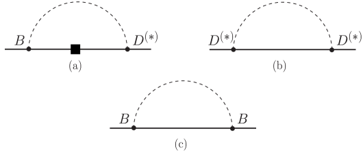
Figure 1: One-loop diagrams that contribute to $B\to D^{*}$. The solid line represents a meson containing a heavy quark, and the dashed line represents light mesons. The small solid circles are strong vertices and contribute a factor of $g_{\pi}$. The large solid square is a weak interaction vertex. Diagram (a) is a vertex correction; (b) and (c) correspond to wavefunction renormalization.

(a)		(b)

Figure 2: Relevant vertices at the quark level. Vertex (a) comes from the LO heavy meson chiral Lagrangian and is proportional to the coefficient $g_{\pi}$. The solid line corresponds to a heavy bottom or charm quark while the dashed lines correspond to light staggered quarks of any flavor and taste. In this vertex, either one or both heavy-light fields must correspond to a vector meson. Vertex (b) comes from the $B\rightarrow D^{(*)}$ operator in Eq. (35). The solid double line corresponds to the bottom quark within the $B$- or $B^{*}$-meson and the solid single line corresponds to the charm quark within the $D$- or $D^{*}$-meson.

	$\;\;+\;\;$		$\;\;+\;\;$		…
		(a)
	$\;\;+\;\;$		$\;\;+\;\;$		…
		(b)
	$\;\;+\;\;$		$\;\;+\;\;$		…
		(c)

Figure 3: Quark flow diagrams that contribute to $B\rightarrow D$ and $B\rightarrow D^{*}$. The double line corresponds to the bottom quark within the $B$-meson, the single line corresponds to the charm quark within the $D^{(*)}$-meson, and the dashed lines correspond to staggered light quarks. Diagram (a) renormalizes the $B$-meson wavefunction while (b) renormalizes the $D^{(*)}$-meson wavefunction. Diagram (c) modifies the $B\rightarrow D^{(*)}$ vertex.

We now present results for the form factors relevant for $B\rightarrow D$ and $B\rightarrow D^{*}$ at zero recoil including taste-breaking effects due to the staggered light quarks.

For the 1+1+1 PQ theory, in which $m_{u}\neq m_{d}\neq m_{s}$:

$$h_{+}^{(B_{x})PQ,1+1+1}(1) = 1+\frac{X_{+}(\Lambda)}{m_{c}^{2}}+\frac{g^{2}_{\pi}}{48\pi^{2}f^{2}}\Bigg{\{}\frac{1}{16}\sum_{\begin{subarray}{l}j=xu,xd,xs\\ \Xi=I,P,4V,4A,6T\end{subarray}}\!\!\!\!\!\!\!{F}_{j_{\Xi}}+\frac{1}{3}\bigg{[}R^{[2,2]}_{X_{I}}\big{(}\{M^{(1)}_{X_{I}}\};\{\mu_{I}\}\big{)}\left(\frac{d{F}_{X_{I}}}{dm^{2}_{X_{I}}}\right)$$ (36)

$$-\sum_{j\in\{M^{(1)}_{I}\}}D^{[2,2]}_{j,X_{I}}\big{(}\{M^{(1)}_{X_{I}}\};\{\mu_{I}\}\big{)}{F}_{j}\bigg{]}+a^{2}\delta^{\prime}_{V}\bigg{[}R^{[3,2]}_{X_{V}}\big{(}\{M^{(3)}_{X_{V}}\};\{\mu_{V}\}\big{)}\left(\frac{d{F}_{X_{V}}}{dm^{2}_{X_{V}}}\right).$$

$$-\sum_{j\in\{M^{(3)}_{V}\}}D^{[3,2]}_{j,X_{V}}\big{(}\{M^{(3)}_{X_{V}}\};\{\mu_{V}\}\big{)}{F}_{j}\bigg{]}+\big{(}V\rightarrow A\big{)}\Bigg{\}},$$

$$h_{A_{1}}^{(B_{x})PQ,1+1+1}(1) = 1+\frac{X_{A}(\Lambda)}{m_{c}^{2}}+\frac{g^{2}_{\pi}}{48\pi^{2}f^{2}}\Big{\{}\frac{1}{16}\sum_{\begin{subarray}{l}j=xu,xd,xs\\ \Xi=I,P,4V,4A,6T\end{subarray}}\!\!\!\!\!\!\!\overline{F}_{j_{\Xi}}+\frac{1}{3}\bigg{[}R^{[2,2]}_{X_{I}}\big{(}\{M^{(1)}_{X_{I}}\};\{\mu_{I}\}\big{)}\left(\frac{d\overline{F}_{X_{I}}}{dm^{2}_{X_{I}}}\right)$$ (37)

$$-\sum_{j\in\{M^{(1)}_{I}\}}D^{[2,2]}_{j,X_{I}}(\{M^{(1)}_{X_{I}}\};\{\mu_{I}\})\overline{F}_{j}\bigg{]}+a^{2}\delta^{\prime}_{V}\bigg{[}R^{[3,2]}_{X_{V}}\big{(}\{M^{(3)}_{X_{V}}\};\{\mu_{V}\}\big{)}\left(\frac{d\overline{F}_{X_{V}}}{dm^{2}_{X_{V}}}\right)$$

$$-\sum_{j\in\{M^{(3)}_{V}\}}D^{[3,2]}_{j,X_{V}}\big{(}\{M^{(3)}_{X_{V}}\};\{\mu_{V}\}\big{)}\overline{F}_{j}\bigg{]}+\big{(}V\rightarrow A\big{)}\Bigg{\}}\,,$$

where $x$ labels the light valence quark within the decaying $B_{x}$ meson. The first term inside the curly braces comes from diagrams with sea quark loops; the flavor index $j$ runs over mesons made of one valence quark and one sea quark and the taste index $\Xi$ runs over the sixteen pion tastes. The residues $R^{[n,k]}_{j}$ and $D^{[n,k]}_{j,l}$ are due to flavor-neutral hairpin propagators; their explicit forms, along with the sets of masses $\{M_{X_{\Xi}}^{(i)}\}$, are given in the Appendix. The second term in the curly braces (with coefficient $1/3$) comes from taste-singlet hairpins, while the third and fourth terms (with coefficients $a^{2}\delta^{\prime}_{V}$ and $a^{2}\delta^{\prime}_{A}$) come from taste-vector and axial-vector hairpins, respectively. The functions $F$ and $\overline{F}$ are defined as

$$F_{j} \equiv F\left(m_{j},\Delta^{(c)}/m_{j}\right)$$ (38)

$$\overline{F}_{j} \equiv F\left(m_{j},-\Delta^{(c)}/m_{j}\right),$$ (39)

where

$$F\left(m_{j},x\right) = \frac{m_{j}^{2}}{x}\bigg{\{}x^{3}\ln\frac{m_{j}^{2}}{\Lambda^{2}}+\frac{1}{3}x^{3}-4x+2\pi$$ (40)

$$-\sqrt{x^{2}-1}(x^{2}+2)\left(\ln\Big{[}1-2x(x-\sqrt{x^{2}-1})\Big{]}-i\pi\right)\bigg{\}}$$

$$\longrightarrow(\Delta^{(c)})^{2}\ln\left(\frac{m_{j}^{2}}{\Lambda^{2}}\right)+{\cal O}[(\Delta^{(c)})^{3}]$$

and $m_{j}$ is the tree-level mass of a meson with flavor-taste index $j$, given in Eq. (20). The analytic terms proportional to $X_{+}(\Lambda)$ and $X_{A}(\Lambda)$ exactly cancel the renormalization scale dependence of the $F$ terms. It is interesting to note that heavy-quark symmetry forbids the presence of additional analytic terms such as those $\propto\textrm{Str}({\cal M})=(m_{u}+m_{d}+m_{s})$ or $\propto a^{2}$. We have checked that these expressions agree with the continuum partially quenched ones when $a\to 0$ Savage (2002). In this limit, the masses of all of the pion tastes become degenerate, so $\frac{1}{16}\sum_{\Xi}F_{j_{\Xi}}\to F_{j}$. Thus the sea quark loop and taste-single hairpin contributions reduce to the continuum PQ result, while the taste-vector and axial-vector contributions, which are proportional to $a^{2}$, vanish.

For the 2+1 theory, in which $m_{u}=m_{d}\neq m_{s}$:

$$h_{+}^{(B_{x})PQ,2+1}(1) = 1+\frac{X_{+}(\Lambda)}{m_{c}^{2}}+\frac{g^{2}_{\pi}}{16\pi^{2}f^{2}}\Bigg{\{}\frac{1}{16}\sum_{\begin{subarray}{l}j=xu,xu,xs\\ \Xi=I,P,4V,4A,6T\end{subarray}}\!\!\!\!\!\!\!F_{j_{\Xi}}+\frac{1}{3}\bigg{[}R^{[2,2]}_{X_{I}}\big{(}\{M^{(5)}_{X_{I}}\};\{\mu_{I}\}\big{)}\left(\frac{dF_{X_{I}}}{dm^{2}_{X_{I}}}\right)$$ (41)

$$-\sum_{j\in\{M^{(5)}_{I}\}}D^{[2,2]}_{j_{I},X_{I}}\big{(}\{M^{(5)}_{X_{I}}\};\{\mu_{I}\}\big{)}F_{X_{I}}\Big{]}+a^{2}\delta^{\prime}_{V}\bigg{[}R^{[3,2]}_{X_{V}}\big{(}\{M^{(7)}_{X_{V}}\};\{\mu_{V}\}\big{)}\left(\frac{dF_{X_{V}},}{dm^{2}_{X_{V}}}\right)$$

$$-\sum_{j\in\{M^{(7)}_{V}\}}D^{[3,2]}_{j_{V},X_{V}}\big{(}\{M^{(7)}_{X_{V}}\};\{\mu_{V}\}\big{)}F_{X_{V}},\bigg{]}+\big{(}V\rightarrow A\big{)}\Bigg{\}},$$

$$h_{A_{1}}^{(B_{x})PQ,2+1}(1) = 1+\frac{X_{A}(\Lambda)}{m_{c}^{2}}+\frac{g^{2}_{\pi}}{48\pi^{2}f^{2}}\Bigg{\{}\frac{1}{16}\sum_{\begin{subarray}{l}j=xu,xu,xs\\ \Xi=I,P,4V,4A,6T\end{subarray}}\!\!\!\!\!\!\!\overline{F}_{j_{\Xi}}$$ (42)

$$+ \frac{1}{3}\bigg{[}R^{[2,2]}_{X_{I}}\big{(}\{M^{(5)}_{X_{I}}\};\{\mu_{I}\}\big{)}\left(\frac{d\overline{F}_{X_{I}}}{dm^{2}_{X_{I}}}\right)-\sum_{j\in\{M^{(5)}_{I}\}}D^{[2,2]}_{j,X_{I}}\big{(}\{M^{(5)}_{X_{I}}\};\{\mu_{I}\}\big{)}\overline{F}_{j}\bigg{]}$$

$$+ a^{2}\delta^{\prime}_{V}\bigg{[}R^{[3,2]}_{X_{I}}\big{(}\{M^{(7)}_{X_{V}}\};\{\mu_{V}\}\big{)}\left(\frac{d\overline{F}_{X_{V}}}{dm^{2}_{X_{V}}}\right)-\sum_{j\in\{M^{(7)}_{V}\}}D^{[3,2]}_{j,X_{V}}\big{(}\{M^{(7)}_{X_{V}}\};\{\mu_{V}\}\big{)}\overline{F}_{j}\Big{]}$$

$$+ \big{(}V\rightarrow A\big{)}\Bigg{\}}.$$

In the case of full (2+1) QCD, the expressions for the residues simplify because QCD is a physical (unitary) theory without double poles:

$$h_{+}^{(B_{u})QCD,2+1}(1) = 1+\frac{X_{+}(\Lambda)}{m_{c}^{2}}+\frac{g^{2}_{\pi}}{16\pi^{2}f^{2}}\left[\frac{1}{16}\sum_{\Xi}\big{(}2F_{\pi_{\Xi}}+F_{K_{\Xi}}\big{)}-\frac{1}{2}F_{\pi_{I}}+\frac{1}{6}F_{\eta_{I}}\right.$$ (43)

$$+a^{2}\delta^{\prime}_{V}\left(\frac{m^{2}_{S_{V}}-m^{2}_{\pi_{V}}}{(m^{2}_{\eta_{V}}-m^{2}_{\pi_{V}})(m^{2}_{\pi_{V}}-m^{2}_{\eta^{\prime}_{V}})}F_{\pi_{V}}+\frac{m^{2}_{\eta_{V}}-m^{2}_{S_{V}}}{(m^{2}_{\eta_{V}}-m^{2}_{\eta^{\prime}_{V}})(m^{2}_{\eta_{V}}-m^{2}_{\pi_{V}})}F_{\eta_{V}}\right.$$

$$\left.\left.+\frac{m^{2}_{S_{V}}-m^{2}_{\eta^{\prime}_{V}}}{(m^{2}_{\eta_{V}}-m^{2}_{\eta^{\prime}_{V}})(m^{2}_{\eta^{\prime}_{V}}-m^{2}_{\pi_{V}})}F_{\eta^{\prime}_{V}}\right)+\big{(}V\rightarrow A\big{)}\right],$$

$$h_{A_{1}}^{(B_{u})QCD,2+1}(1) = 1+\frac{X_{A}(\Lambda)}{m_{c}^{2}}+\frac{g^{2}_{\pi}}{48\pi^{2}f^{2}}\left[\frac{1}{16}\sum_{\Xi}\big{(}2\overline{F}_{\pi_{\Xi}}+\overline{F}_{K_{\Xi}}\big{)}-\frac{1}{2}\overline{F}_{\pi_{I}}+\frac{1}{6}\overline{F}_{\eta_{I}}\right.$$ (44)

$$+a^{2}\delta^{\prime}_{V}\left(\frac{m^{2}_{S_{V}}-m^{2}_{\pi_{V}}}{(m^{2}_{\eta_{V}}-m^{2}_{\pi_{V}})(m^{2}_{\pi_{V}}-m^{2}_{\eta^{\prime}_{V}})}\overline{F}_{\pi_{V}}+\frac{m^{2}_{\eta_{V}}-m^{2}_{S_{V}}}{(m^{2}_{\eta_{V}}-m^{2}_{\eta^{\prime}_{V}})(m^{2}_{\eta_{V}}-m^{2}_{\pi_{V}})}\overline{F}_{\eta_{V}}\right.$$

$$\left.\left.+\frac{m^{2}_{S_{V}}-m^{2}_{\eta^{\prime}_{V}}}{(m^{2}_{\eta_{V}}-m^{2}_{\eta^{\prime}_{V}})(m^{2}_{\eta^{\prime}_{V}}-m^{2}_{\pi_{V}})}\overline{F}_{\eta^{\prime}_{V}}\right)+\big{(}V\rightarrow A\big{)}\right].$$

$$h_{+}^{(B_{s})QCD,2+1}(1) = 1+\frac{X_{+}(\Lambda)}{m_{c}^{2}}+\frac{g^{2}_{\pi}}{16\pi^{2}f^{2}}\left[\frac{1}{16}\sum_{\Xi}\big{(}F_{S_{\Xi}}+2F_{K_{\Xi}}\big{)}-F_{S_{I}}+\frac{2}{3}F_{\eta_{I}}\right.$$ (45)

$$+a^{2}\delta^{\prime}_{V}\left(\frac{m^{2}_{S_{V}}-m^{2}_{\pi_{V}}}{(m^{2}_{S_{V}}-m^{2}_{\eta_{V}})(m^{2}_{S_{V}}-m^{2}_{\eta^{\prime}_{V}})}F_{S_{V}}+\frac{m^{2}_{\eta_{V}}-m^{2}_{\pi_{V}}}{(m^{2}_{\eta_{V}}-m^{2}_{S_{V}})(m^{2}_{\eta_{V}}-m^{2}_{\eta^{\prime}_{V}})}F_{\eta_{V}}\right.$$

$$\left.\left.+\frac{m^{2}_{\eta^{\prime}_{V}}-m^{2}_{\pi_{V}}}{(m^{2}_{\eta^{\prime}_{V}}-m^{2}_{S_{V}})(m^{2}_{\eta^{\prime}_{V}}-m^{2}_{\eta_{V}})}F_{\eta^{\prime}_{V}}\right)+\big{(}V\rightarrow A\big{)}\right],$$

$$h_{A_{1}}^{(B_{s})QCD,2+1}(1) = 1+\frac{X_{A_{1}}(\Lambda)}{m_{c}^{2}}+\frac{g^{2}_{\pi}}{48\pi^{2}f^{2}}\left[\frac{1}{16}\sum_{\Xi}\big{(}\overline{F}_{S_{\Xi}}+2\overline{F}_{K_{\Xi}}\big{)}-\overline{F}_{S_{I}}+\frac{2}{3}\overline{F}_{\eta_{I}}\right.$$ (46)

$$+a^{2}\delta^{\prime}_{V}\left(\frac{m^{2}_{S_{V}}-m^{2}_{\pi_{V}}}{(m^{2}_{S_{V}}-m^{2}_{\eta_{V}})(m^{2}_{S_{V}}-m^{2}_{\eta^{\prime}_{V}})}\overline{F}_{S_{V}}+\frac{m^{2}_{\eta_{V}}-m^{2}_{\pi_{V}}}{(m^{2}_{\eta_{V}}-m^{2}_{S_{V}})(m^{2}_{\eta_{V}}-m^{2}_{\eta^{\prime}_{V}})}\overline{F}_{\eta_{V}}\right.$$

$$\left.\left.+\frac{m^{2}_{\eta^{\prime}_{V}}-m^{2}_{\pi_{V}}}{(m^{2}_{\eta^{\prime}_{V}}-m^{2}_{S_{V}})(m^{2}_{\eta^{\prime}_{V}}-m^{2}_{\eta_{V}})}\overline{F}_{\eta^{\prime}_{V}}\right)+\big{(}V\rightarrow A\big{)}\right],$$

Note that there are separate formulae for $B_{u,d}\rightarrow D^{(*)}_{u,d}$ and $B_{s}\rightarrow D^{(*)}_{s}$ in full QCD. This is in contrast to the PQ expressions, which are valid for any choice of light quark flavor. These results agree with the continuum full QCD ones when $a\to 0$ Randall and Wise (1993); Savage (2002).

IV Numerical Illustration of the $B\to D^{*}$ Form Factor

In this section we present a realistic picture of the behavior of staggered lattice data for $B\to D^{*}$ and compare our S$\chi$PT expression to actual staggered lattice data for $B\to D$.

Figure 4, which shows the full QCD expression for $h_{A_{1}}(1)$ vs. $m_{\pi}^{2}$, illustrates the importance of accounting for staggered discretization errors in the extrapolation of staggered lattice data. There are currently no unquenched staggered lattice data for $B\to D^{*}$ available, so we have added a term linear in $m_{\pi}^{2}$ to the S$\chi$PT expression for $h_{A_{1}}(1)$ and matched onto existing quenched data simulated at heavy ($>500\mathop{\rm MeV}\nolimits$) pion masses Hashimoto et al. (2002). Thus Figure 4 gives a realistic illustration of what the chiral extrapolation of unquenched data for $h_{A_{1}}(1)$ from the MILC coarse lattices ($a=0.125$ fm) might look like. The continuum expression for $h_{A_{1}}(1)$ has a characteristic cusp at $m_{\pi}=\Delta_{c}$ where the internal $D$ goes on-shell. The staggered expression has a cusp in the same location due to the taste pseudoscalar pion, which receives no taste-breaking shifts to its mass, but the cusp is much milder.

It is worthwhile to discuss in some detail why the staggered cusp is so mild, or, equivalently, how the staggered curve in Figure 4 becomes the continuum curve when $a\rightarrow 0$. A cusp occurs in $h_{A_{1}}$ every time the internal pion and $D$ go on-shell in the $B\to D^{*}$ diagram. For a staggered pion of taste $\Xi$, this happens when $m_{\pi}^{2}+a^{2}\Delta_{\Xi}=\Delta_{c}^{2}$, where $m_{\pi}^{2}$ is the tree-level mass of the lattice Goldstone pion and $a^{2}\Delta_{\Xi}$ is the taste-breaking mass correction. Thus, in Figure 4, there is a cusp in the staggered curve every time $m_{\pi}^{2}=\Delta_{c}^{2}-a^{2}\Delta_{\Xi}$. On the MILC coarse lattices, all of the ${\cal O}(a^{2})$ mass-splittings are greater than $\Delta_{c}=0.14\mathop{\rm GeV}\nolimits$, so the additional heavy staggered pions do not produce cusps in Figure 4. The single staggered cusp due to the lattice Goldstone pion is small because it is weighted by $1/16$ (from the average over pion tastes in the loop) as compared to the continuum one. As the lattice spacing is reduced, more and more tastes will be able to produce cusps to the left of the continuum one. These cusps will begin at $m_{\pi}^{2}=0$ and move to the right as the lattice spacing becomes smaller. Finally, at $a=0$, all of the cusps from the non-Goldstone pions will come to rest at the location of the continuum one, and the sum of these sixteen staggered cusps will equal the single cusp in the continuum curve. In addition to softening the cusp, the heavy staggered pions decrease the curvature due to chiral logarithms in $h_{A_{1}}$; this is a generic effect of taste-breaking. Thus the staggered data are expected to be almost linear, even when the continuum result is not.

In practice, one extrapolates staggered lattice data to the continuum by first fitting to Eq. (44) and then removing taste-breaking discretization errors by setting the terms proportional to $a^{2}$ in Eq. (44) to zero. We note that simulations are not likely to be sensitive to the cusp anytime soon, even if staggering did not smooth it out, because the cusp only occurs at values very close to the physical pion mass. Thus, in the case of $B\to D^{*}$, it is especially important to use S$\chi$PT to extrapolate to the physical light quark masses.

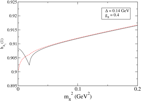
Figure 4: Qualitative behavior of $h_{A_{1}}(1)$ vs. $m_{\pi}^{2}$. The overall linear contribution comes from matching to existing quenched data Hashimoto et al. (2002). The curve with the large cusp is the continuum expression, whereas the (dashed) curve with the mild cusp includes staggered discretization effects. We use the measured values of the pion mass-splittings and taste-breaking hairpins from the MILC coarse lattices as input into the staggered curve Aubin et al. (2004).

We can also directly apply our S$\chi$PT expression to the available unquenched data for $B\to D$ Okamoto et al. (2005). Figure 5 shows $h_{+}(1)$ vs. $m_{\pi}^{2}$ in full QCD. In this case, the pion and $D^{*}$ in the loops of the diagrams of Figure 1 cannot go on-shell, so there is no cusp as in the case of $B\to D^{*}$. The dashed line is the result of a fit of the staggered expression to the three data points. The solid line is the continuum extrapolated curve, while the square is the continuum extrapolated value of $h_{+}(1)$ at the physical value of the pion mass, with error bars. The difference between these curves is very small, and the extrapolated value hardly differs from the result of a naive linear fit. Nevertheless, the S$\chi$PT analysis is useful for this quantity because it demonstrates that the systematic errors associated with the chiral extrapolation are small.

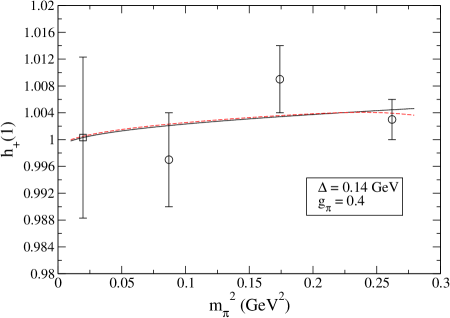
Figure 5: $h_{+}(1)$ vs. $m_{\pi}^{2}$. The three full QCD data points (circles) were calculated on the MILC coarse lattices ($a=0.125$ fm) Okamoto et al. (2005). The upper (dashed) curve is a fit to the data using the complete staggered formula, while the lower (solid) curve is the continuum extrapolated curve. The square is the extrapolated value of $h_{+}(1)$ at the physical pion mass with error bars.

V Finite Volume Effects in $B\to D^{(*)}$

The functions $F$ and $\bar{F}$, which appear in $h_{+}(1)$ and $h_{A_{1}}(1)$, respectively, are modified by the finite spatial extent of the lattice. Using the formulae for finite volume corrections to typical HM$\chi$PT integrals given in Ref. Arndt and Lin (2004), we find that $F(m,\Delta)$ receives the following correction due to the finite lattice volume:

$$\delta F_{FV}(m,\Delta,\textrm{L}) = \sum_{\vec{n}\neq\vec{0}}\left(\frac{m^{2}}{128xy^{3}}\right)e^{-y}\Bigg{\{}\pi e^{x^{2}y/2}\bigg{[}y^{5}x^{12}-(y-16)y^{4}x^{10}$$ (47)

$$+2(y+24)y^{3}x^{8}-16(y-2)y^{3}x^{6}+96y^{3}x^{4}-128y^{3}x^{2}+256y^{2}\bigg{]}$$

$$+\sqrt{2\pi y}\bigg{[}-y^{4}x^{11}+(y-15)y^{3}x^{9}-(3y+35)y^{2}x^{7}$$

$$+(16y^{2}-27y+15)yx^{5}+(-112y^{2}+11y-9)x^{3}+256y^{2}x\bigg{]}$$

$$-256\pi y^{2}-\pi y^{2}e^{x^{2}y/2}\textrm{erf}\left(\frac{x\sqrt{y}}{\sqrt{2}}\right)\bigg{[}y^{3}x^{12}-(y-16)y^{2}x^{10}$$

$$+2(y+24)yx^{8}-16(y-2)yx^{6}+96yx^{4}-128yx^{2}+256\bigg{]}\Bigg{\}},$$

where $x=\Delta/m$ as before, $y=nm\textrm{L}$, and $n=\sqrt{\vec{n}^{2}}$. The correction to $\bar{F}$ is identical except for $x\to-x$. This formula was derived as a series expansion in $1/(nm\textrm{L})$. In our numerical evaluation of this formula we truncate the sum to the values of $n=1$, $\sqrt{2}$, $\sqrt{3}$, $\sqrt{4}$, $\sqrt{5}$ and $\sqrt{6}$. An expansion in $x=\Delta/m$ shows that the leading contribution to $\delta F_{FV}$ is proportional to $\Delta^{2}$, as expected:

$$\delta F_{FV}(m,\Delta,\textrm{L}) = \sum_{\vec{n}\neq\vec{0}}\sqrt{\frac{\pi}{2}}\left(\frac{m^{2}x^{2}}{192y^{5/2}}\right)e^{-y}\left(128y^{3}-336y^{2}+33y-27\right)+{\cal O}(x^{3}).$$ (48)

Figure 6 shows the contribution to $h_{+}(1)$ in full QCD from finite volume effects for the MILC coarse lattice ($a=0.125$ fm, $\textrm{L}=2.5$ fm). Recall from Figure 5 that $h_{+}(1)$ is close to one, whereas the finite volume corrections in Figure 6 are less than $10^{-4}$ in the range of pion masses relevant for current staggered lattice simulations. The size of finite volume corrections to $h_{A_{1}}(1)$ are similarly small. We therefore conclude that finite volume errors are negligible in both the $B\to D$ and $B\to D^{*}$ form factors, and can be accounted for as an overall systematic error in lattice calculations, rather than subtracted before the chiral extrapolation.

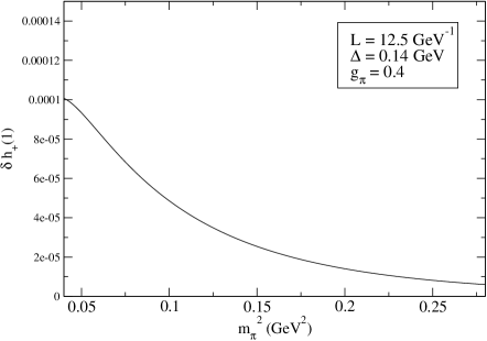
Figure 6: Finite volume correction to $h_{+}(1)$ as a function of $m_{\pi}^{2}$. Recall that $h_{+}(1)$ is close to 1, so these corrections are smaller than one part in $10^{-4}$ in current staggered simulations.

VI Conclusions

In this work we have calculated the $B\to D$ and $B\to D^{*}$ form factors at zero recoil to NLO in S$\chi$PT. We have presented expressions for both a “1+1+1” partially quenched theory ($m_{u}\neq m_{d}\neq m_{s}$) and a “2+1” partially quenched theory ($m_{u}=m_{d}\neq m_{s}$), as well as for full (2+1) QCD. These formulae apply to simulations in which only the light quark is staggered. They include ${\cal O}(a^{2})$ taste-breaking discretization errors, and are necessary for correct continuum and chiral extrapolation of staggered $B\to D^{(*)}$ lattice data. Use of these expressions, along with the double ratio method of Ref. Hashimoto et al. (2002) and in combination with experimental input, should allow a precise determination of the CKM matrix element $|V_{cb}|$.

APPENDIX

In this section we collect formulae necessary for understanding our form factor results. We follow the notation of Ref. Aubin and Bernard (2003b).

The residues $R^{[n,k]}_{j}$ and $D^{[n,k]}_{j,l}$ appear because of single and double poles, respectively, in the flavor-neutral hairpin propagators:

$$R^{[n,k]}_{j}(\{m\},\{\mu\}) \equiv \frac{\prod_{a=1}^{k}(\mu^{2}_{a}-m^{2}_{j})}{\prod_{i\neq j}(m^{2}_{i}-m^{2}_{j})},$$

$$D^{[n,k]}_{j,l}(\{m\},\{\mu\}) \equiv -\frac{d}{dm^{2}_{l}}R^{[n,k]}_{j}(\{m\},\{\mu\}).$$ (A1)

Once one takes the mass of the overall flavor-taste singlet pion (which corresponds to the physical $\eta^{\prime}$) to infinity, the relationships among the taste-singlet pion masses simplify:

$$m^{2}_{\pi_{I}} = m^{2}_{U_{I}}=m^{2}_{D_{I}},$$

$$m^{2}_{\eta_{I}} = \frac{m^{2}_{U_{I}}}{3}+\frac{2m^{2}_{S_{I}}}{3},$$ (A2)

Thus the following mass combinations appear in the 1+1+1 ($m_{u}\neq m_{d}\neq m_{s}$) PQ result:

$$\{M_{X}^{(1)}\} \equiv \{m_{\pi^{0}},m_{\eta},m_{X}\},$$

$$\{M_{X}^{(3)}\} \equiv \{m_{\pi^{0}},m_{\eta},m_{\eta^{\prime}},m_{X}\},$$

$$\{\mu\} \equiv \{m_{U},m_{D},m_{S}\}$$ (A3)

When the up and down quark masses are degenerate, the pion mass eigenstates become:

$$m^{2}_{\pi_{V}} = m^{2}_{U_{V}}=m^{2}_{D_{V}},$$

$$m^{2}_{\eta_{V}} = \frac{1}{2}\left(m^{2}_{U_{V}}+m^{2}_{S_{V}}+\frac{3}{4}a^{2}\delta^{\prime}_{V}-Z\right),$$

$$m^{2}_{\eta^{\prime}_{V}} = \frac{1}{2}\left(m^{2}_{U_{V}}+m^{2}_{S_{V}}+\frac{3}{4}a^{2}\delta^{\prime}_{V}+Z\right),$$

$$Z \equiv \sqrt{(m^{2}_{S_{V}}-m^{2}_{U_{V}})^{2}-\frac{a^{2}\delta^{\prime}_{V}}{2}(m^{2}_{S_{V}}-m^{2}_{U_{V}})+\frac{9(a^{2}\delta^{\prime}_{V})^{2}}{16}},$$ (A4)

Thus the following mass combinations appear in the 2+1 ($m_{u}=m_{d}\neq m_{s}$) PQ result:

$$\{M_{X}^{(5)}\} \equiv \{m_{\eta},m_{X}\},$$

$$\{M_{X}^{(7)}\} \equiv \{m_{\eta},m_{\eta^{\prime}},m_{X}\},$$

$$\{\mu\} \equiv \{m_{U},m_{S}\}$$ (A5)

References

Hashimoto et al. (2000)
S. Hashimoto
et al., Phys. Rev.
D61, 014502
(2000), eprint hep-ph/9906376.
Hashimoto et al. (2002)
S. Hashimoto,
A. S. Kronfeld,
P. B. Mackenzie,
S. M. Ryan, and
J. N. Simone,
Phys. Rev. D66,
014503 (2002), eprint hep-ph/0110253.
Okamoto et al. (2005)
M. Okamoto et al.,
Nucl. Phys. Proc. Suppl. 140,
461 (2005), eprint hep-lat/0409116.
Kennedy (2005)
A. D. Kennedy,
Nucl. Phys. Proc. Suppl. 140,
190 (2005), eprint hep-lat/0409167.
Aubin et al. (2004)
C. Aubin et al.
(MILC), Phys. Rev.
D70, 114501
(2004), eprint hep-lat/0407028.
Lee and Sharpe (1999)
W.-J. Lee and
S. R. Sharpe,
Phys. Rev. D60,
114503 (1999), eprint hep-lat/9905023.
Aubin and Bernard (2003a)
C. Aubin and
C. Bernard,
Phys. Rev. D68,
034014 (2003a),
eprint hep-lat/0304014.
Aubin and Bernard (2003b)
C. Aubin and
C. Bernard,
Phys. Rev. D68,
074011 (2003b),
eprint hep-lat/0306026.
Sharpe and Van de Water (2005)
S. R. Sharpe and
R. S. Van de Water,
Phys. Rev. D71,
114505 (2005), eprint hep-lat/0409018.
Aubin and Bernard (2005)
C. Aubin and
C. Bernard
(2005), eprint hep-lat/0510088.
Aubin et al. (2005)
C. Aubin et al.,
Phys. Rev. Lett. 95,
122002 (2005), eprint hep-lat/0506030.
Laiho (2005)
J. Laiho (2005),
eprint hep-lat/0510058.
Arndt and Lin (2004)
D. Arndt and
C. J. D. Lin,
Phys. Rev. D70,
014503 (2004), eprint hep-lat/0403012.
Kronfeld (2000)
A. S. Kronfeld,
Phys. Rev. D62,
014505 (2000), eprint hep-lat/0002008.
Kronfeld (2004)
A. S. Kronfeld,
Nucl. Phys. Proc. Suppl. 129,
46 (2004), eprint hep-lat/0310063.
Burdman and Donoghue (1992)
G. Burdman and
J. F. Donoghue,
Phys. Lett. B280,
287 (1992).
Wise (1992)
M. B. Wise,
Phys. Rev. D45,
2188 (1992).
Sharpe and Zhang (1996)
S. R. Sharpe and
Y. Zhang,
Phys. Rev. D53,
5125 (1996), eprint hep-lat/9510037.
Isgur and Wise (1989)
N. Isgur and
M. B. Wise,
Phys. Lett. B232,
113 (1989).
Luke (1990)
M. E. Luke,
Phys. Lett. B252,
447 (1990).
Dürr (2005)
S. Dürr,
Proc. Sci. LAT2005,
021 (2005), eprint hep-lat/0509026.
Savage (2002)
M. J. Savage,
Phys. Rev. D65,
034014 (2002), eprint hep-ph/0109190.
Randall and Wise (1993)
L. Randall and
M. B. Wise,
Phys. Lett. B303,
135 (1993), eprint hep-ph/9212315.