Probing the Aoki phase with $N_{f}=2$ Wilson fermions at finite temperature

Abstract

In this letter we report on a numerical investigation of the Aoki phase in the case of finite temperature which continues our former study at zero temperature. We have performed simulations with Wilson fermions at $\beta=4.6$ using lattices with temporal extension $N_{\tau}=4$. In contrast to the zero temperature case, the existence of an Aoki phase can be confirmed for a small range in $\kappa$ at $\beta=4.6$, however, shifted slightly to lower $\kappa$. Despite fine-tuning $\kappa$ we could not separate the thermal transition line from the Aoki phase.

I Introduction

The interest in the phase structure of Wilson fermions coupled to $SU(3)$ gauge fields has revived recently, in particular due to the unexpected discovery of a first-order transition in twisted mass QCD Farchioni et al. (2005a). This transition survives when the Wilson gauge action is replaced by a renormalization group improved gauge action Farchioni et al. (2005b). This has brought reports on a nontrivial phase structure  Blum et al. (1994); Aoki et al. (2004) back into the center of interest including the pioneering paper by Aoki Aoki (1984).

The Aoki phase, characterized by a non-vanishing condensate $\langle\bar{\psi}i\gamma_{5}\tau^{3}\psi\rangle$ and a broken pion mass triplet, was analyzed in the framework of chiral perturbation theory in Sharpe and Singleton (1998); Münster (2004). In Münster (2004) two scenarios were described: at a given gauge coupling $\beta$ either the Aoki phase is realized in a certain $\kappa$ interval (separated by second order phase transition lines from a phase with degenerate massive pions), or there are first order transitions in a certain interval of twisted masses (also ending at second order transition points).

In a recent paper Ilgenfritz et al. (2004) we have found evidence that the Aoki phase at zero temperature is unlikely to extend to $\beta>4.6$, whereas the mentioned new phase transition has been observed at $\beta=5.2$ Farchioni et al. (2005a). The change between those two scenarios seems to happen between these two values of $\beta$.

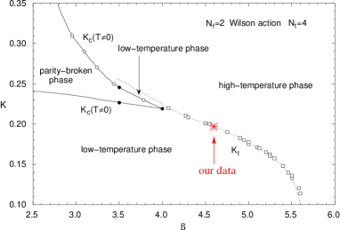
Figure 1: The phase diagram with Wilson fermions at finite temperature as presented in Aoki et al. (1996). We have added a point at $\beta=4.6$ where we have found evidence for the Aoki phase.

From the very beginning it was interesting to know where the Aoki phase lies at finite temperature. Numerical studies Aoki et al. (1996); Aoki (1998) have given some indications that the Aoki phase is completely embedded in the low temperature phase as proposed by Aoki et al. Aoki et al. (1996). Their results for $N_{f}=2$ and $N_{\tau}=4$ are shown in Fig. 1. However, the results left open the question, whether the Aoki phase will join the thermal transition line $K_{T}(\beta,N_{\tau})$ as it extends further in $\beta$ for a given thermal lattice extension $N_{\tau}$.

To be specific, the following observations were made by Aoki et al. Aoki et al. (1996) for $N_{f}=2$ dynamical flavors: For $N_{\tau}=4$ at $\beta=3.5$ (on a $8^{3}\times 4$ lattice) a finite parity-flavor breaking condensate $\langle\bar{\psi}i\gamma_{5}\tau^{3}\psi\rangle$ was found in a $\kappa$ interval where $m_{\pi^{\pm}}=0$. Surprisingly, the cusp of the Aoki phase moved slightly towards larger $\beta$ when $N_{\tau}$ is increased. In fact, going from $N_{\tau}=4$ to $N_{\tau}=8$ resulted only in a shift from $\beta=4.0$ to $\beta=4.2$. At larger $\beta$ no evidence for the Aoki phase — at finite temperature — has been found in unquenched simulations so far.

In a finite-temperature study by the MILC collaboration on a $12^{3}\times 6$ lattice Blum et al. (1994) metastabilities of plaquette values at ($\beta,\kappa$) =(4.8,0.19), (5.02,0.18) and (5.22,0.17) were found. This observation could be compatible with the metastability at (5.20, 0.1715) observed in Farchioni et al. (2005a).

A possible scenario could be that the tip of the cusp simply stops moving and turns into a first order line along which $m_{\pi}\neq 0$, separating phases with $m_{q}<0$ (at high $\kappa$) from $m_{q}>0$ (at low $\kappa$) Creutz (1996); Ukawa .

What happens to the first order phase transition line at weaker coupling? Is it universal and how does this affect the continuum limit? Does the transition extend to $\beta\to\infty$ as a single first order line? Or does it split again giving room for a new Aoki-like phase enclosed? Can the Aoki phase extend towards $\beta\to\infty$ being enclosed by two second order lines using improved actions?

II Numerical results

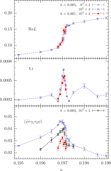
Figure 2: The real part of the Polyakov loop, its susceptibility $\chi_{L}$ and the order parameter $\langle\bar{\psi}i\gamma_{5}\tau^{3}\psi\rangle$ as a function of $\kappa$ at $h=0.005$ and 0.001 fixed. The lower panels shows $h=0.003$ additionally. The data have been obtained from simulations on a $8^{3}\times 4$ and a $10^{3}\times 4$ lattice at $\beta=4.6$. Throughout the same symbols are used.

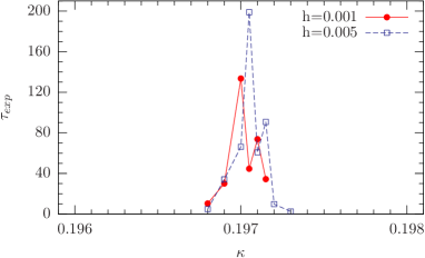
Figure 3: The (exponential) autocorrelation time $\tau_{exp}$ (in terms of HMC trajectories) of the real part of the Polyakov loop is shown as a function of $\kappa$ for two different values of $h$. The lattice size is $10^{3}\times 4$.

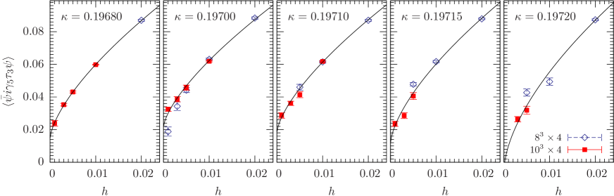
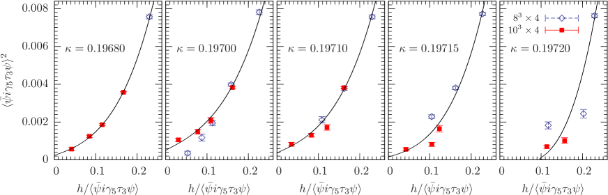
Figure 4: The upper panels show the order parameter $\langle\bar{\psi}i\gamma_{5}\tau^{3}\psi\rangle$ as a function of $h$ at five values of $\kappa$. The lines are fits to the data as described in the text. The lower panels show Fisher plots of the order parameter and the corresponding fitting function at the same values of $\kappa$ as above. Throughout the same symbols are used.

$\kappa$	$h=0.001$		$h=0.003$		$h=0.005$		$h=0.010$		$h=0.020$
0.19680	$10^{3}\times 4$	1000	$10^{3}\times 4$	1000	$10^{3}\times 4$	1100	$8^{3}\times 4$	1000	$8^{3}\times 4$	90
0.19690	$10^{3}\times 4$	1600	$10^{3}\times 4$	2000	$10^{3}\times 4$	1600	$8^{3}\times 4$	1500	$8^{3}\times 4$	60
0.19700	$10^{3}\times 4$	2500	$10^{3}\times 4$	4100	$8^{3}\times 4$	3900	$10^{3}\times 4$	1000	$8^{3}\times 4$	150
0.19705	$10^{3}\times 4$	1900	$10^{3}\times 4$	1800	$10^{3}\times 4$	4800	$10^{3}\times 4$	1700	$8^{3}\times 4$	400
0.19710	$10^{3}\times 4$	3200	$10^{3}\times 4$	3000	$10^{3}\times 4$	3400	$10^{3}\times 4$	1700	$8^{3}\times 4$	150
0.19715	$10^{3}\times 4$	2000	$10^{3}\times 4$	1000	$10^{3}\times 4$	2500	$8^{3}\times 4$	300	$8^{3}\times 4$	200
0.19720			$10^{3}\times 4$	400	$10^{3}\times 4$	400	$8^{3}\times 4$	500	$8^{3}\times 4$	300

Table 1: Statistics used for the final analysis at selected $\kappa$ at $\beta=4.6$.

$\kappa$	fit	A	B	C	D	E	$\chi^{2}/\textsc{ndf}$	fit	A	B	C	D	E	$\chi^{2}/\textsc{ndf}$
	1	0.015(1)	1	0.67(1)	0	0	0.24	2	0.016(1)	1.07(7)	0.69(2)	0	0	0.24
$0.19680$	3	0.026(1)	1	0.68(1)	0.1(1)	0	0.23	4	0.015(1)	1	0.68(1)	0	2(2)	0.19
	1	0.021(1)	1	0.70(1)	0	0	0.57	2	0.022(2)	0.73(4)	0.73(4)	0	0	0.65
$0.19690$	3	0.022(2)	1	0.72(2)	0.2(2)	0	0.64	4	0.022(1)	1	0.71(1)	0	4(4)	0.59
	1	0.022(2)	1	0.70(1)	0	0	2.48	2	0.026(1)	1.5(2)	0.81(3)	0	0	0.56
$0.19700$	3	0.026(2)	1	0.76(3)	0.6(2)	0	0.59	4	0.025(2)	1	0.72(1)	0	11(4)	0.87
	1	0.019(2)	1	0.68(1)	0	0	4.0	2	0.023(4)	1.2(3)	0.74(7)	0	0	4.3
$0.19705$	3	0.022(3)	1	0.72(4)	0.3(3)	0	4.3	4	0.022(3)	1	0.70(2)	0	5(6)	4.2
	1	0.019(2)	1	0.68(1)	0	0	2.48	2	0.017(2)	0.9(3)	0.66(9)	0	0	3.54
$0.19710$	3	0.017(5)	1	0.67(4)	-0.1(4)	0	3.49	4	0.017(4)	1	0.67(2)	0	-4(8)	3.31
	1	0.012(3)	1	0.66(1)	0	0	4.74	2	0.008(9)	0.6(1)	0.84(3)	0	0	6.26
$0.19715$	3	0.008(8)	1	0.63(6)	-0.3(6)	0	6.26	4	0.009(6)	1	0.64(3)	0	-9(13)	5.8
	1	-0.005(6)	1	0.61(2)	0	0	5.16	2	0.019(10)	7(1)	1.2(4)	0	0	6.26
$0.19720$	3	0.015(10)	1	1(27)	3(41)	0	0.65	4	0.014(2)	1	0.77(3)	0	60(8)	0.14

Table 2: The parameters of the ansatz $~{}\sigma(h)=A+Bh^{C}+Dh+Eh^{2}~{}$ fitted to the data of $\langle\bar{\psi}i\gamma_{5}\tau^{3}\psi\rangle$ at $\beta=4.6$ without (fits labeled 1 and 2), with linear, or with quadratic corrections (labeled 3 and 4). At each $h$ the result from the largest lattice was used in the fit (for details see Table 1). Fixed parameters are given by their value without indicating an error. In each case the first fit (bold numbers) was used in Fig. 4.

In this study we looked for the Aoki phase at finite temperature at $\beta$ larger than in earlier studies. We performed numerical simulations at temporal lattice extension $N_{\tau}\equiv 4$ using dynamical unimproved Wilson fermions. The Wilson fermion matrix $M_{W}$ was supplemented by an explicit parity-flavor symmetry breaking term, i.e. the two-flavor fermion matrix was given by

$$M(h)=M_{W}+h\,i\gamma_{5}\tau^{3}.$$ (1)

We simulated at $\beta=4.6$. $\kappa$ was fine-tuned in the interval $[0.193,0.199]$ at fixed values of $h$. For each triple $(\beta,\kappa,h)$ the order parameter $\langle\bar{\psi}i\gamma_{5}\tau^{3}\psi\rangle$, the real part of Polyakov loop $\mathop{\mathrm{Re}L}$ and its susceptibility $\chi_{\textrm{L}}$ were measured. These observables are shown in Fig. 2. From the Figure we see that $\mathop{\mathrm{Re}L}$ and $\chi_{\textrm{L}}$ reveal a finite temperature transition around $\kappa=0.19705$, while the order parameter $\langle\bar{\psi}i\gamma_{5}\tau^{3}\psi\rangle$ signals an existence of the Aoki phase in this $\kappa$ region.

Note that we had found a vestigial region around $\kappa\approx 0.1984$ at $\beta=4.6$ in our previous zero-temperature study Ilgenfritz et al. (2004). Therefore, the Aoki phase seems to follow the finite-temperature transition line and is shifted to somewhat lower $\kappa$ compared to the zero-temperature case. This shift, however, cannot be resolved in Fig. 1. In any case, the Aoki phase extends inside a longer cusp than seen in Aoki et al. (1996).

In the region of interest around $\kappa=0.19705$ we found rather long autocorrelations in the Monte Carlo time histories in contrast to other $\kappa$ values. The autocorrelation function has been estimated for the Polyakov loop and we found large values for the exponential $\tau_{exp}$ and the integrated autocorrelation time $\tau_{int}$ (in terms of HMC trajectories). Examples for $\tau_{exp}$ at $h=0.005$ and 0.001 are shown in Fig. 3.

In order to study the Aoki phase, the limit

$$\langle\bar{\psi}i\gamma_{5}\tau^{3}\psi\rangle_{h=0}=\lim_{h\rightarrow 0}\lim_{V\rightarrow\infty}\langle\bar{\psi}i\gamma_{5}\tau^{3}\psi\rangle$$ (2)

has to be taken. Therefore, we made runs in the interval $\kappa\in[0.1968,0.19720]$ at several values of $h\in[0.001,0.02]$ using spatial volumes $8^{3}$ and $10^{3}$.

In the upper panels of Fig. 4 the results of those simulations are shown together with fits to the data from the largest lattice available at each $h$. For the fits we used the ansatz Ilgenfritz et al. (2004)

$$\sigma(h)=A+Bh^{C}+\ldots\quad,$$ (3)

where $\sigma\equiv\langle\bar{\psi}i\gamma_{5}\tau^{3}\psi\rangle$. The value of the order parameter at $h=0$ is given by the fit parameter $A$. The fits are quite robust against the introduction of linear and quadratic corrections. Details of the statistics achieved are presented in Tab. 1. We did not list the information refering to the smaller lattice size $8^{3}\times 4$ in all those cases, where $10^{3}\times 4$ data were available. The results of all our fits are quoted in Tab. 2.

The lower panels of Fig. 4 show the same results as in the upper panels, however, in a different parametrization (so called Fisher plots, see e.g. Kouvel and Fisher (1964); Göckeler et al. (1997); Ilgenfritz et al. (2004)). This parametrization has the advantage that the curves bend upwards, if $\langle\bar{\psi}i\gamma_{5}\tau^{3}\psi\rangle$ is non-zero in the limit $h\rightarrow 0$. Hence, the finiteness of the intercept point can be read off better. In addition, it enables us to see directly if this intercept grows with the volume. At $\kappa=0.19700$ we have computed the order parameter at lower values of $h$ also for the smaller lattice size $8^{3}\times 4$. As expected, a clear volume dependence is found, indicating that the existence of the Aoki phase becomes visible only for sufficient large volumes. The right most panels of Fig. 4 show data at ($\kappa=0.19720$) to illustrated a case where the order parameter $\langle\bar{\psi}i\gamma_{5}\tau^{3}\psi\rangle$ is found to vanish.

III Discussion

By measuring the order parameter $\langle\bar{\psi}i\gamma_{5}\tau^{3}\psi\rangle$ and extrapolating it to $h=0$ we conclude that there is a parity-flavor broken phase at finite temperature ($N_{\tau}=4$) at $\beta=4.6$ in the interval $0.1968\leq\kappa\leq 0.19715$. In the zero-temperature case we had found Ilgenfritz et al. (2004) that the Aoki phase seems to end in the vicinity of $\beta=4.6$, $\kappa=0.1984$. In other words, for a finite temperature the endpoint of the Aoki phase is shifted towards larger $\beta$ and also to lower $\kappa$.

This result differs from Aoki et al. (1996); Aoki (1998) where the endpoint of the Aoki phase for $N_{\tau}=4$ was seen at $\beta=4.0$, $\kappa=0.22$. The finite-temperature transition line determined in Refs. Aoki et al. (1996); Aoki (1998) crosses the interval $\beta=4.6$, $0.1968\leq\kappa\leq 0.19715$ in which we see the Aoki phase. Although we have studied the respective $\kappa$ interval in rather small steps, we are not able to separate (the boundary of) the Aoki phase from the thermal phase transition (cf. Fig. 1). We plan to extend our investigation to larger $N_{\tau}$ values in the near future.

References

- Farchioni et al. (2005a) F. Farchioni et al., Eur. Phys. J. C39, 421 (2005a), eprint hep-lat/0406039.
- Farchioni et al. (2005b) F. Farchioni et al., Eur. Phys. J. C42, 73 (2005b), eprint hep-lat/0410031.
- Blum et al. (1994) T. Blum et al., Phys. Rev. D50, 3377 (1994), eprint hep-lat/9404006.
- Aoki et al. (2004) S. Aoki et al. (JLQCD) (2004), eprint hep-lat/0409016.
- Aoki (1984) S. Aoki, Phys. Rev. D30, 2653 (1984).
- Sharpe and Singleton (1998) S. R. Sharpe and J. Singleton, Robert, Phys. Rev. D58, 074501 (1998), eprint hep-lat/9804028.
- Münster (2004) G. Münster, JHEP 09, 035 (2004), eprint hep-lat/0407006.
- Ilgenfritz et al. (2004) E.-M. Ilgenfritz, W. Kerler, M. Müller-Preussker, A. Sternbeck, and H. Stüben, Phys. Rev. D69, 074511 (2004), eprint hep-lat/0309057.
- Aoki et al. (1996) S. Aoki, A. Ukawa, and T. Umemura, Phys. Rev. Lett. 76, 873 (1996), eprint hep-lat/9508008.
- Aoki (1998) S. Aoki, Nucl. Phys. Proc. Suppl. 60A, 206 (1998), eprint hep-lat/9707020.
- Creutz (1996) M. Creutz (1996), eprint hep-lat/9608024.
- (12) A. Ukawa, talk given at the workshop Lattice QCD simulations via International Research Network, Shuzenji, Japan, 21–24 September 2004, URL http://www.ccs.tsukuba.ac.jp/workshop/ilft04/presen/InformalWorkshop/Ukawa.pdf.
- Kouvel and Fisher (1964) J. S. Kouvel and M. E. Fisher, Phys. Rev. 136, A1626 (1964).
- Göckeler et al. (1997) M. Göckeler et al., Nucl. Phys. B487, 313 (1997), eprint [http://arXiv.org/abs]hep-lat/9605035.