Landau gauge ghost and gluon propagators in $SU(2)$ lattice gauge theory: Gribov ambiguity revisited

Abstract

We reinvestigate the problem of Gribov ambiguities within the Landau (or Lorentz) gauge for the ghost and gluon propagators in pure $SU(2)$ lattice gauge theory. We make use of the full symmetry group of the action taking into account large, i.e. non-periodic $\mathbb{Z}(2)$ gauge transformations leaving lattice plaquettes invariant. Enlarging in this way the gauge orbits for any given gauge field configuration the Landau gauge can be fixed at higher local extrema of the gauge functional in comparison with standard (overrelaxation) techniques. This has a clearly visible effect not only for the ghost propagator at small momenta but also for the gluon propagator, in contrast to the common belief.

I Introduction

It is an important task to compute (Landau or Coulomb) gauge gluon, ghost, fermion propagators and the basic vertex functions from non-perturbative approaches to $SU(N)$ gauge theories, like Dyson-Schwinger equations or the lattice formulation. On one hand one is interested in their behavior in the infrared limit in order to extract non-perturbative informations on various observables, e.g. the QCD running couplings $\alpha_{s}(q^{2})$, to understand quark and gluon confinement within the Gribov-Zwanziger scenario Gribov (1978); Zwanziger (1994, 2004), or to check the Kugo-Ojima confinement criterion for the absence of colored states Kugo and Ojima (1979). On the other hand it is technically important to see to what extent these different non-perturbative approaches provide results consistent with each other in the non-perturbative region, i.e. at low momenta. At present we are still far from drawing final conclusions in this respect. In particular the Dyson-Schwinger approach Alkofer and von Smekal (2001); Fischer and Alkofer (2003); Lerche and von Smekal (2002), always relying on a truncated set of equations, provides results which look quite different in the infinite volume limit compared with those obtained on a torus Fischer et al. (2002); Fischer and Alkofer (2002); Fischer et al. (2005), while the latter show at least qualitative agreement with recent results of numerical lattice simulations Sternbeck et al. (2005a).

It is well known that gauge fixing in the non-perturbative range is faced with the Gribov ambiguity problem, which means that there can be many gauge copies for a given gauge field satisfying the Landau gauge condition $~{}\partial_{\mu}A_{\mu}=0~{}$ within the Gribov region, the latter defined by the positivity of the Landau gauge Faddeev-Popov operator. In recent years one has checked in greater detail how strong Gribov copies can influence the infrared behavior especially of the gluon and ghost propagators. Several groups of authors came to the conclusion that while there is a clearly visible influence on the ghost propagator, the gluon propagator seems only weakly affected Cucchieri (1997); Bakeev et al. (2004); Nakajima and Furui (2004); Silva and Oliveira (2004); Sternbeck et al. (2005a).

Recently Zwanziger has argued that in the infinite volume limit the influence of Gribov copies: “… might be negligible, i.e. all averages taken over the Gribov region should become equal to averages over the fundamental modular region” Zwanziger (2004). However, in practical lattice simulations we are always restricted to finite volumes. Thus, Gribov copies have to be taken into account properly before extrapolating to the infrared and infinite volume.

In this paper we present a reinvestigation of the Gribov copy problem for the $SU(2)$ case. The usual way to fix the (Landau) gauge on the lattice is to simulate the path integral in its gauge invariant form. Subsequently each of the produced lattice gauge fields $~{}U\equiv\{U_{x,\mu}\}~{}$ is subjected to an iterative procedure maximizing the gauge functional

$$F(g) = \frac{1}{dV}\sum_{x,\mu}\frac{1}{2}\mbox{Tr}~{}U^{g}_{x,\mu}\,,$$

$$U^{g}_{x,\mu} = g(x)~{}U_{x,\mu}~{}g^{\dagger}(x+{\hat{\mu}})$$ (1)

with respect to local gauge transformations $~{}g\equiv\{g(x)\in SU(2)\}$. $~{}V=L^{d}~{}$ denotes the number of lattice sites in $~{}d=4~{}$ dimensions. The local maxima of $~{}F(g)~{}$ satisfy the differential lattice Landau gauge transversality condition

$$(\partial_{\mu}A^{g}_{\mu})(x)=A^{g}_{\mu}(x+{\hat{\mu}}/2)-A^{g}_{\mu}(x-{\hat{\mu}}/2)=0\,,$$ (2)

where the lattice gauge potentials are

$$A_{\mu}(x+{\hat{\mu}}/2)=\frac{1}{2i}(U_{x,\mu}-U_{x,\mu}^{\dagger})\,.$$ (3)

The standard procedure assumes periodic gauge transformations and employs the overrelaxation algorithm. In what follows we shall abbreviate it by SOR. The influence of Gribov copies can be easily studied by taking various initial random gauge copies of the gauge field configurations before subjecting them to the SOR algorithm.

At this place it is worth to note that the widely - at least till now - accepted approach to compute e.g. a gauge-variant propagator $G$ is to choose always the gauge copy with the highest value of local maxima $F_{max}$ (or the best copy) found for the gauge functional (1). One can then hope to have found a copy belonging to the so-called fundamental modular region or at least being not far from it. In order to find the best copy for each thermalized gauge field configuration one needs to compare $F_{max}$-values for a pretty large amount of gauge copies, which is a rather time consuming procedure. A reasonable question is if the use of only one gauge copy (the first copy) provides us with the same - within errorbars - values of the propagator as the use of the best copy. This logic brings us to compare the propagator calculated on best copies ($G^{(bc)}$) with that on the first copies ($G^{(fc)}$). The relative deviation $~{}\delta G\equiv|(G^{(fc)}-G^{(bc)})/G^{(bc)}|~{}$ provides then a useful quantitive measure of the Gribov ambiguity of the quantity under consideration. We shall discuss this measure throughout the present paper.

Of course, one can enhance the effect of Gribov copies by comparing instead the best copies with the worst copies, i.e. with those having the smallest values $F_{max}$ found from the repeated use of a given maximization method. This attitude has been taken in Ref. Silva and Oliveira (2004) in order to highlight a Gribov copy effect for the gluon propagator.

In Refs. Bakeev et al. (2004) for $SU(2)$ and Sternbeck et al. (2005a) for $SU(3)$ some of us already have thoroughly discussed the impact of Gribov copies within the SOR framework by comparing first and best copies. From this point of view the gluon propagator did not depend on the copies within the statistical noise, whereas the ghost propagator clearly was depending on them in the infrared. But the data for the ghost propagator obtained for different lattice sizes showed an indication for a weakening of the dependence on the choice of Gribov copies for increasing lattice size at fixed momentum, in agreement with Zwanziger’s claim Zwanziger (2004).

Here we enlarge the class of possible gauge transformations by taking into account also non-periodic center gauge transformations. This will allow us to maximize further the gauge functional and to see a quite strong Gribov copy effect also for the gluon propagator at finite (lattice) volumes.

In Sec. II we shall explain the improved gauge fixing procedure. In Sec. III we define the propagators to be calculated. In Sec. IV we are going to present our results for the gluon and ghost propagators, whereas in Sec. V the conclusions will be drawn.

II Improved gauge fixing

We shall deal all the time with $SU(2)$ pure gauge lattice fields in four Euclidean dimensions produced by means of Monte Carlo simulations with the standard Wilson plaquette action. We restrict ourselves to the confinement phase at $T=0$.

To fix the gauge we employ the standard Los Alamos type overrelaxation with $\omega=1.7$.

Our generalization of the standard gauge fixing procedure SOR comes from the simple observation that gauge covariance for periodic $SU(2)$ gauge fields on a $d$-dimensional torus of extension $L^{d}$ allows gauge transformations which are not necessarily periodic but can differ by a group center element at the boundary:

$$g(x+L\hat{\nu})=z_{\nu}g(x)\,,z_{\nu}=\pm 1\in\mathbb{Z}(2)\,.$$ (4)

In light of this it is legitimate to allow, during the maximization of the gauge functional in the gauge fixing procedure, for gauge tranformations which differ by a sign when winding around a boundary. Let $\nu$ be the direction of such boundary. Any such gauge transformation can be decomposed into a standard periodic gauge transformation (which we may call a “small” one) and a flip of all links $~{}U_{\nu}(x)\to-~{}U_{\nu}(x)~{}$ of a 3-plane at a given fixed $~{}x_{\nu}$. Given a “small” random gauge copy of the configuration we have thus performed a pre-conditioning step for the gauge functional by sweeping in every direction all 3-planes in succession and comparing the value of the flipped with the unflipped gauge functional. The flip is accepted if the gauge functional increases. It is easy to see that such a procedure is independent of the order of choosing the 3-planes and that only one sweep through the lattice is required to maximize the functional. The gauge copy obtained at the end of this procedure is then used as a starting point for a standard maximization procedure. We call the whole procedure FOR.

Analogously to the SOR method the FOR procedure can be repeated with different initial random gauges in order to find a best copy ( bc ) in comparison e.g. with the first random copy ( fc ). We shall check the convergence of the  bc -propagator results for the best copies as a function of the number $~{}n_{copy}~{}$ of random initial copies.

III Gluon and ghost propagators

We turn now to the computation of the gauge variant gluon and ghost propagators within the Landau gauge.

The lattice gluon propagator $~{}D^{ab}_{\mu\nu}(p)~{}$ is taken as the Fourier transform of the gluon two-point function, i.e. the expectation value

$$D^{ab}_{\mu\nu}(p) = \left\langle\widetilde{A}^{a}_{\mu}(\hat{k})\widetilde{A}^{b}_{\nu}(-\hat{k})\right\rangle_{U}$$

$$= \delta^{ab}\left(\delta_{\mu\nu}-\frac{p_{\mu}~{}p_{\nu}}{p^{2}}\right)D(p)\,.$$

$\widetilde{A}^{a}_{\mu}(\hat{k})~{}$ is the Fourier transform of the lattice gauge potential $~{}A^{a}_{\mu}(x+\hat{\mu}/2)$. $~{}p~{}$ denotes the four-momentum

$$p_{\mu}(\hat{k}_{\mu})=\frac{2}{a}\sin\left(\frac{\pi\hat{k}_{\mu}}{L}\right)$$ (6)

with the integer-valued lattice momentum $~{}\hat{k}_{\mu}\in(-L/2,+L/2]$. $a$ is the lattice spacing.

The lattice ghost propagator is defined by inverting the Faddeev-Popov (F-P) operator, the latter being the Hessian of the gauge functional Eq. (1). The F-P operator can be written in terms of the (gauge-fixed) link variables $~{}U_{x,\mu}~{}$ as

$$M^{ab}_{xy}=\sum_{\mu}A^{ab}_{x,\mu}\,\delta_{x,y}-B^{ab}_{x,\mu}\,\delta_{x+\hat{\mu},y}-C^{ab}_{x,\mu}\,\delta_{x-\hat{\mu},y}\quad$$ (7)

with

$$A^{ab}_{x,\mu} = \frac{1}{2}~{}\delta_{ab}~{}\mbox{Tr}\left[U_{x,\mu}+U_{x-\hat{\mu},\mu}\right]\,,$$

$$B^{ab}_{x,\mu} = \frac{1}{2}~{}\mbox{Tr}\left[\sigma^{b}\sigma^{a}\,U_{x,\mu}\right]\,,$$

$$C^{ab}_{x,\mu} = \frac{1}{2}~{}\mbox{Tr}\left[\sigma^{a}\sigma^{b}\,U_{x-\hat{\mu},\mu}\right]\,,$$

where the $~{}\sigma^{a}\,,a=1,2,3~{}$ are the Pauli matrices. In the continuum $~{}M^{ab}_{xy}~{}$ corresponds to the operator $~{}M^{ab}=-\partial_{\mu}D^{ab}_{\mu}$, with $~{}D^{ab}~{}$ the covariant derivative in the adjoint representation.

The ghost propagator in momentum space is calculated from the ensemble average

$$G^{ab}(p) = \frac{1}{V}\sum_{x,y}\left\langle{\rm e}^{-2\pi i\,\hat{k}\cdot(x-y)}[M^{-1}]^{a\,b}_{x\,y}\right\rangle_{U}$$ (8)

$$= \delta^{ab}~{}G(p)\,.$$ (9)

Following Ref. Suman and Schilling (1996); Cucchieri (1997) we have used the conjugate gradient (CG) algorithm to invert $~{}M~{}$ on a plane wave $~{}\vec{\psi}_{c}=\{~{}\delta_{ac}\exp(2\pi i\,\hat{k}\!\cdot\!x)~{}\}$.

After solving $~{}M\vec{\phi}=\vec{\psi}_{c}~{}$ the resulting vector $~{}\vec{\phi}~{}$ is projected back on $~{}\vec{\psi}~{}$ so that the average $~{}G^{cc}(p)~{}$ over the color index $~{}c~{}$ can be taken explicitly. Since the F-P operator $~{}M~{}$ is zero if acting on constant modes, only $~{}\hat{k}\neq(0,0,0,0)~{}$ is permitted. Due to high computational requirements to invert the F-P operator for each $~{}\hat{k}$, separately, the estimators on a single, gauge-fixed configuration are evaluated only for a preselected set of momenta $~{}\hat{k}$.

IV Results

We consider various bare couplings in the interval $~{}\beta=4/g_{0}^{2}~{}\in[2.1,2.5]~{}$ and lattice sizes up to $~{}20^{4}~{}$. We compare the gluon and ghost propagators obtained with the alternative gauge fixing methods SOR (‘flips off’) and FOR (‘flips on’) both for the first ( fc ) and best copy ( bc ). In order to find the best copies we always generate $~{}20~{}$ initial random gauge copies.

 

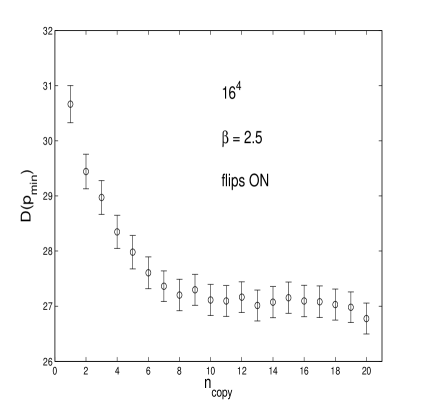
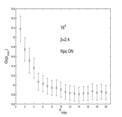
Figure 1: Gluon propagator (left) and ghost propagator (right) at lowest momentum $~{}p_{min}=(2/a)\sin(\pi/L)~{}$ versus number of random copies employing the FOR method (’flips on’) at $~{}\beta=2.5~{}$ and $~{}2.4$, respectively (lattice size $~{}16^{4}~{}$).

In Fig. 1 we illustrate for the FOR method how fast the gluon and ghost propagators are converging when determined from the best copy out of the first $~{}n_{copy}~{}$ copies. We see plateaus occuring for $~{}n_{copy}\geq O(10)$. We have convinced ourselves that $~{}O(20)~{}$ copies are sufficient at least for $\beta\geq 2.3$ and lattice sizes up to $20^{4}$. For the SOR method the convergence is faster - although to worse values of the gauge functional - such that in principle a smaller number of copies would be sufficient within the given parameter range.

Mostly we have concentrated on the lowest non-trivial on-axis lattice momentum $~{}p_{min}~{}=~{}(2/a)\sin(\pi/L)~{}$ and some multiple on-axis momenta in order to study the infrared limit for given lattice size and bare coupling. We are aware of the fact that this choice is by far too restrictive in order to get reliable results for the (renormalized) propagators in the continuum and thermodynamic limit.

 

Figure 2: Gluon propagator $~{}D(p_{min})~{}$ at lowest momentum for various $~{}\beta~{}$ and for lattice sizes $~{}12^{4}~{}$ (left) and $~{}16^{4}~{}$ (right). Full dots refer to FOR  fc  and open squares (circles) correspond to SOR  fc  ( bc ).

 

Figure 3: Ghost propagator $~{}G(p_{min})~{}$ as for Fig. 2.

In Fig. 2 and Fig. 3 we show our results for the lattice gluon $D(p_{min})$ and ghost propagators $G(p_{min})$ for $12^{4}$ and $16^{4}$ lattices, always for the smallest non-vanishing momentum. In order to demonstrate the effect of the $\mathbb{Z}(2)$ flips in comparison with the SOR results obtained with  bc  and  fc  copies Bakeev et al. (2004) we show three sets of data points: black dots correspond to FOR - ‘flips on’ and  bc  copies and open circles (squares) correspond to SOR - ‘flips off’ for  bc  ( fc ) copies. The corresponding data are listed in Table 1.

$12^{4}$ $\beta$ $\#$ $D_{\rm{FOR}}^{(bc)}$ $\#$ $D_{\rm{SOR}}^{(bc)}$ $D_{\rm{SOR}}^{(fc)}$ 2.10 1200 $5.39(6)$ 900 $5.79(8)$ $5.83(8)$ 2.20 1200 $7.94(9)$ 1200 $8.74(10)$ $8.66(10)$ 2.30 1200 $12.16(14)$ 1200 $12.69(15)$ $12.85(15)$ 2.40 3600 $15.10(10)$ 2080 $17.06(17)$ $17.12(17)$ 2.44 5100 $15.13(9)$ 2.47 5700 $14.64(9)$ 2.50 2650 $14.16(13)$ 1760 $17.34(26)$ $17.42(26)$ $16^{4}$ $\beta$ $\#$ $D_{\rm{FOR}}^{(bc)}$ $\#$ $D_{\rm{SOR}}^{(bc)}$ $D_{\rm{SOR}}^{(fc)}$ 2.10 1042 $5.59(7)$ 918 $5.93(8)$ $5.95(8)$ 2.20 900 $9.01(12)$ 740 $9.35(14)$ $9.58(14)$ 2.30 1100 $14.88(18)$ 510 $16.16(31)$ $15.97(29)$ 2.40 1032 $22.65(29)$ 1020 $24.36(32)$ $25.03(32)$ 2.45 1020 $25.69(32)$ 1030 $28.19(36)$ $28.21(38)$ 2.50 1040 $26.86(35)$ 1060 $30.64(44)$ $30.37(45)$       $12^{4}$ $\beta$ $\#$ $G_{\rm{FOR}}^{(bc)}$ $\#$ $G_{\rm{SOR}}^{(bc)}$ $G_{\rm{SOR}}^{(fc)}$ 2.10 1200 $11.58(4)$ 900 $11.87(4)$ $12.48(7)$ 2.20 1200 $10.10(8)$ 1200 $10.39(3)$ $10.90(5)$ 2.30 1200 $8.37(2)$ 1200 $8.99(6)$ $9.27(4)$ 2.40 3600 $7.04(1)$ 2080 $7.80(3)$ $7.97(4)$ 2.44 5100 $6.65(1)$ 2.47 5700 $6.36(1)$ 2.50 2650 $6.11(1)$ 1760 $7.26(5)$ $7.40(5)$ $16^{4}$ $\beta$ $\#$ $G_{\rm{FOR}}^{(bc)}$ $\#$ $G_{\rm{SOR}}^{(bc)}$ $G_{\rm{SOR}}^{(fc)}$ 2.10 1042 $22.89(6)$ 918 $23.12(13)$ $24.15(8)$ 2.20 900 $19.83(6)$ 740 $20.29(6)$ $21.34(9)$ 2.30 1100 $16.83(5)$ 510 $17.27(8)$ $18.05(10)$ 2.40 1032 $14.00(4)$ 1020 $14.88(6)$ $15.60(8)$ 2.45 1020 $12.92(5)$ 1030 $13.86(6)$ $14.41(11)$ 2.50 1040 $12.02(4)$ 1060 $13.26(6)$ $13.45(7)$

Table 1: Data for the gluon propagator $D(p)$ (left) as well as for the ghost propagator $G(p)$ (right) at lowest momentum $p=p_{min}$ obtained with FOR ( bc ) and SOR ( bc  and  fc ) methods on $12^{4}$ and $16^{4}$ lattices.

We clearly see that the FOR method leads to an additional visible Gribov copy effect not only for the ghost propagator but also for the gluon propagator. The effect is even more pronounced at higher $\beta$-values, i.e. at smaller ’physical’ lattice sizes. We have convinced ourselves that this is compatible with the behavior of the average maximal gauge functional $\langle F_{max}\rangle$. Its relative difference determined with  bc  copies for the FOR method versus the SOR method is also rising with $\beta$. Later on we shall see that this observation is also in one-to-one correspondence with the gauge copy dependence for fixed $\beta$ and varying lattice size. The anatomy of the (new) FOR gauge copies deserves further studies in the future.

In order to illustrate the strong Gribov copy effect in a slightly different manner we compare smoothed distributions for the mean value estimators for the gluon and ghost propagators for the  bc  with the FOR and SOR method, respectively (see Fig. 4). The mean value distributions have been obtained in accordance with the bootstrap method Efron and Tibshirani (1993) from replica of sequences of randomly selected data. Such bootstrapped resampling was applied to the initial MC data set as a whole, the amount of replicas being typically 200. To smoothen the distribution we have used the standard Nadaraya–Watson method with normal kernel Bowman and Azzalini (1997), and an improved Silverman’s rule of thumb for the choice of the corresponding bandwidth.

It is worth mentioning that the statistical errors for most of our data have also been estimated through bootstrapped resampling.

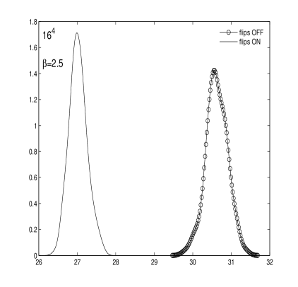
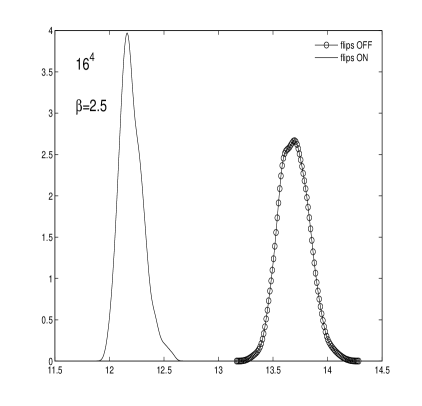
Figure 4: SOR- and FOR-distributions for $D^{(bc)}(p_{min})$ (left) and $G^{(bc)}(p_{min})$ (right) at $\beta=2.5$ and $16^{4}$ lattice.

We have also studied how the Gribov copy effect develops for larger momenta $p(\hat{k})$. We have used multiples of the minimal lattice momentum $\hat{k}=(0,0,0,k),~{}k=1,2,3,4~{}$ along one axis. We compare for the gluon propagator the  bc  SOR results with  bc  FOR results in terms of the relative deviation

$$\delta D(p)=(D_{\rm{SOR}}^{(bc)}-D_{\rm{FOR}}^{(bc)})/D_{\rm{FOR}}^{(bc)}~{},$$ (10)

and analogously for the ghost propagator $~{}G(p)~{}$ at various $\beta$-values and with fixed lattice size $~{}16^{4}~{}$ (see Fig. 5). For the gluon propagator our results are restricted to only one $\beta$-value because of the much stronger statistical noise. Nevertheless, the results presented for the gluon propagator point into the same direction as for the ghost propagator. The effect of Gribov copies still remains noticable at $p>p_{min}$, although decreasing for rising momenta.

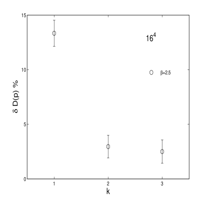
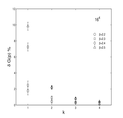
Figure 5: Left: relative deviation $~{}\delta D(p)=(D_{\rm{SOR}}^{(bc)}-D_{\rm{FOR}}^{(bc)})/D_{\rm{FOR}}^{(bc)}~{}$ in percent for the gluon propagator at various (on-axis) lattice momenta $~{}p(k)~{}$ (lattice size $16^{4}$, $\beta=2.5$).
Right: the analogous relative deviation for the ghost propagator for the same lattice size but for $\beta=2.2,2.3,2.4$ and $2.5$.

The data for the ghost propagator at various momenta obtained from independent Monte Carlo runs are also collected in Table 2.

FOR
$\beta$	$\#$		$G(k=1)$	$G(k=2)$	$G(k=3)$	$G(k=4)$
2.20	400	fc	21.2(1)	3.96(1)	1.510(2)	0.8116(5)
		bc	19.88(8)	3.868(7)	1.493(1)	0.8076(4)
2.30	400	fc	18.2(2)	3.39(3)	1.313(2)	0.7276(6)
		bc	16.88(8)	3.267(6)	1.299(1)	0.7241(4)
2.40	356	fc	15.4(1)	2.87(1)	1.171(1)	0.6693(3)
		bc	13.8(1)	2.770(8)	1.156(2)	0.6647(4)
2.50	400	fc	13.7(1)	2.578(5)	1.0897(8)	0.6357(2)
		bc	12.2(1)	2.508(5)	1.079(1)	0.6325(3)
SOR
$\beta$	$\#$		$G(k=1)$	$G(k=2)$	$G(k=3)$	$G(k=4)$
2.20	200	fc	21.2(2)	3.97(2)8	1.511(3)	0.8117(7)
		bc	20.23(12)	3.885(10)	1.4971(25)	0.8084(7)
2.30	200	fc	18.2(1)	3.35(1)	1.312(2)	0.7272(5)
		bc	17.3(1)	3.297(8)	1.304(1)	0.7253(5)
2.40	370	fc	15.6(1)	2.87(1)	1.171(1)	0.6690(3)
		bc	14.8(1)	2.83(1)	1.165(1)	0.6673(3)
2.50	200	fc	14.1(2)	2.586(8)	1.090(1)	0.6359(4)
		bc	13.4(1)	2.564(6)	1.088(1)	0.6352(3)

Table 2: Ghost propagators $G(p)$ on the $16^{4}$ lattice for various on-axis lattice momenta $~{}p(k)$.

We have also made a corresponding check for the gluon propagator at zero momentum. On a lattice of size $20^{4}$ and for the same $\beta=2.5$ we observed a deviation between the  bc  FOR and SOR results of the order $O(25\%)$. This would of course have consequences for estimates like in Ref. Bonnet et al. (2001); Boucaud et al. (2006), since the infinite volume extrapolation of $D(0)$ there performed, although probably remaining finite, will definitely suffer from uncontrolled systematic uncertainties.

It is interesting to study the volume dependence of the Gribov copy effect, in view of Zwanziger’s recent claim mentioned at the beginning Zwanziger (2004).

Figure 6: Distributions of the number of different gauge copies found with the FOR method at $\beta=2.40$ for lattice sizes $8^{4}$ and $16^{4}$.

Figure 7: Distributions of the deviation of the gauge functional values for different gauge copies relative to the best copy per configuration. FOR method at $\beta=2.40$ for lattice sizes $8^{4}$ and $16^{4}$.

Figure 8: Distributions of ghost propagator values at lowest non-trivial momentum for different gauge copies as in Fig. 7.

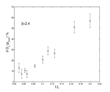
Figure 9: Relative deviation $~{}\delta D_{L}(p_{min})~{}\equiv~{}(D_{\rm{SOR}}^{(fc)}-D_{\rm{FOR}}^{(bc)})/D_{\rm{FOR}}^{(bc)}~{}$ in percent for the gluon propagator $~{}D~{}$ for various linear lattice sizes $~{}L~{}$ and smallest non-vanishing momentum $~{}p_{min}~{}=~{}(2/a)\sin(\pi/L)~{}$ ($\beta=2.4$).

First of all we have convinced ourselves that the number of gauge copies is strongly rising with the lattice volume as it should be. This is clearly demonstrated in Fig. 6 providing the distributions of the number of gauge copies per configuration found with the FOR method (‘flips on’) for lattice sizes $8^{4}$ and $16^{4}$ at $\beta=2.40$. In both cases we have generated 100 configurations with 100 gauge copies each. It turns out that identical (or degenerated) copies can be well recognized at an accuracy for the gauge functional Eq. (1) of $O(10^{-10})$. Adjacent copies normally differ in the values for the gauge functional at a level of $O(10^{-6})$. Now let us compare the distributions of the corresponding values of the functional $F$ for each copy found. In order to normalize the values with respect to the highest (i.e. best) value per configuration we show the relative deviation $(F_{max}^{(bc)}-F_{max})/F_{max}^{(bc)}$. The frequency distributions of these values are shown in Fig. 7 for the same ensembles as used for Fig. 6. There is a very clear tendency that the variance of the gauge functional becomes much smaller if we increase the lattice volume. A similar tendency becomes visible in Fig. 8, where we plot for the same set of configurations and gauge copies the distributions for the single values of the ghost propagator for the lowest non-vanishing on-axis momentum. Also in this case we have normalized the single values as $(G^{(bc)}-G)/G^{(bc)}$, i.e. taking the relative deviation of the propagator at a given copy $G$ from the value computed on the best copy $G^{bc}$, the latter chosen again with respect to the gauge functional value. We see that the long tail seen for the smaller lattice disappears for the larger lattice. Although the fact that close values of the gauge functional will not tell anything about how much the corresponding gauge configurations are differing from each other (irrespective of a global relative gauge transformation) we would like to interprete our finding of shrinking distributions as a weakening of the Gribov problem with increasing ’physical’ lattice size.

Moreover, we have plotted the relative deviation

$$\delta D_{L}(p_{min})~{}\equiv(D_{\rm{SOR}}^{(fc)}-D_{\rm{FOR}}^{(bc)})/D_{\rm{FOR}}^{(bc)}$$ (11)

for the gluon propagator (see Fig. 9) and analogously for the ghost propagator (see l.h.s. of Fig. 10) as a function of the inverse linear lattice size $~{}1/L~{}$, both determined at the minimal momentum $~{}p_{min}$. Here we have used data for fixed $~{}\beta=2.4~{}$ and lattice sizes from $~{}L=5~{}$ up to $~{}L=20$. In close correspondence to our observations presented in Figs. 2 and 3 we see that the Gribov copy effect becomes weaker (stronger) for increasing (decreasing) ’physical’ lattice size and correspondingly decreasing (increasing) minimal momentum, at least up to a certain value of the lattice size ($\mbox{}_{\textstyle\sim}^{\textstyle<}15$). One would of course need larger values of $L$ to make a reliable conclusion about the limit $L\to\infty$. Anyway, at our largest lattice value $L=20$ the Gribov copy effect is still quite strong.

For the ghost propagator, where the signal to noise ratio is more favourable, we have found an analogous behavior also for the multiple on-axis momenta $~{}k=2,3,4$ (see r.h.s. of Fig. 10).

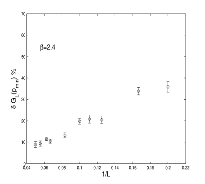
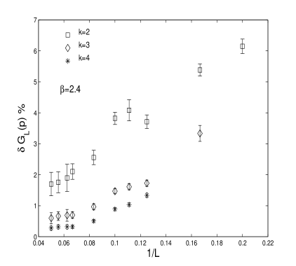
Figure 10: Relative deviation $~{}\delta G_{L}(p)~{}\equiv~{}(G_{\rm{SOR}}^{(fc)}-G_{\rm{FOR}}^{(bc)})/G_{\rm{FOR}}^{(bc)}~{}$ in percent for the ghost propagator $~{}G~{}$ at $\beta=2.4$ for various linear lattice sizes $~{}L~{}$ and the smallest non-vanishing momentum $~{}p_{min}~{}=~{}(2/a)\sin(\pi/L)~{}$ (left) as well as for on-axis momenta $~{}p(k),~{}k=2,3,4$ (right).

In Bakeev et al. (2004) two of us have reported on rare Monte Carlo events with exceptionally large values of the ghost propagator occuring for the SOR gauge fixing method for larger $~{}\beta$ values. In Fig. 11 we show some time histories for the gluon and ghost propagators for $\beta=2.5$ and a $16^{4}$ lattice, comparing  bc  SOR with  bc  FOR. We see that for the ‘best copy - flips on’ case (FOR) the fluctuations for both propagators are smaller. But for the ghost propagator the effect of exceptionally large values, in general related to small eigenvalues of the F-P operator Sternbeck et al. (2005b), is still there.

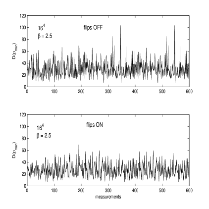
Figure 11: Time histories for $D^{(bc)}(p_{min})$ (left) and $G^{(bc)}(p_{min})$ (right) for both SOR and FOR methods at $\beta=2.5$ and $16^{4}$ lattice.

Concluding we show the form factors of the gluon propagator $~{}p^{2}D(p)~{}$ and of the ghost propagator $~{}p^{2}G(p)~{}$ in physical units as a function of the physical momentum for fixed $~{}\beta=2.4~{}$ and lattice sizes varying from $~{}10^{4}~{}$ to $~{}20^{4}~{}$. We have rescaled the gluon propagator values $~{}D(p)~{}$ with factors $~{}a^{2}~{}$ and $~{}g_{0}^{2}~{}$ and the ghost propagator $~{}G(p)~{}$ with $~{}a^{2}~{}$, respectively, in order to translate to the corresponding continuum (bare) propagators (compare with Bloch et al. (2004)). To estimate the lattice spacing in physical units we have used the string tension: $~{}a^{2}\sigma=.071~{}$ Fingberg et al. (1993) with the standard value $~{}\sqrt{\sigma}=440\mathrm{MeV}$. The form factor results for both methods  bc  SOR and  bc  FOR are shown together in Fig. 12. Again the figure shows clear Gribov copy effects for both the propagators and not only for the ghost propagator. We did not apply any overall renormalization here. The statistics collected for these runs is listed in Table 3.

FOR
$L$	5	6	8	9	10	12	15	16	18	20
$N_{conf}$	1000	1000	800	600	600	500	400	356	200	200
SOR
$L$	5	6	8	9	10	12	15	16	18	20
$N_{conf}$	1000	1000	800	500	500	400	400	370	100	100

Table 3: Statistics for the measurements at different $L$ and $\beta=2.4$.

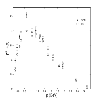
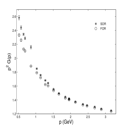
Figure 12: Gluon form factor $~{}p^{2}D(p)~{}$ (left) and ghost form factor $~{}p^{2}G(p)~{}$ (right) both for the  bc  SOR and  bc  FOR methods versus momentum obtained for various lattice sizes and fixed $~{}\beta=2.4$.

V Conclusions

In this paper we have demonstrated that there is a visible Gribov problem for the ghost propagator as well as for the gluon propagator computed in $SU(2)$ lattice gauge theory within the Landau gauge. In order to show this we have enlarged the gauge orbits of given Monte Carlo generated gauge fields by non-periodic $\mathbb{Z}(2)$ transformations, flipping all links in a given direction on a slice orthogonal to that. This allows a preconditioning which maximizes the gauge functional before applying the overrelaxation algorithm.

We have found indications for a weakening of the Gribov copy effect both going to larger momenta at fixed volume and also increasing the lattice size $L$ while correspondingly lowering the minimal non-zero momentum, at least up to a certain value of the lattice size ($\mbox{}_{\textstyle\sim}^{\textstyle<}15$). However, one would need larger values of $L$ to draw a reliable conclusion about the limit $L\to\infty$.

We have not shown the momentum scheme running coupling which can be determined from the form factors of the propagators discussed here assuming that the renormalization factor for the ghost-gluon vertex is constant. This will be discussed in a future paper, where we want to present data for larger lattices and a larger spectrum of (off-axis) momenta.

References

- Gribov (1978) V. N. Gribov, Nucl. Phys. B139, 1 (1978).
- Zwanziger (1994) D. Zwanziger, Nucl. Phys. B412, 657 (1994).
- Zwanziger (2004) D. Zwanziger, Phys. Rev. D69, 016002 (2004), eprint hep-ph/0303028.
- Kugo and Ojima (1979) T. Kugo and I. Ojima, Prog. Theor. Phys. Suppl. 66, 1 (1979).
- Alkofer and von Smekal (2001) R. Alkofer and L. von Smekal, Phys. Rept. 353, 281 (2001), eprint hep-ph/0007355.
- Fischer and Alkofer (2003) C. S. Fischer and R. Alkofer, Phys. Rev. D67, 094020 (2003), eprint hep-ph/0301094.
- Lerche and von Smekal (2002) C. Lerche and L. von Smekal, Phys. Rev. D65, 125006 (2002), eprint hep-ph/0202194.
- Fischer et al. (2002) C. S. Fischer, R. Alkofer, and H. Reinhardt, Phys. Rev. D65, 094008 (2002), eprint hep-ph/0202195.
- Fischer and Alkofer (2002) C. S. Fischer and R. Alkofer, Phys. Lett. B536, 177 (2002), eprint hep-ph/0202202.
- Fischer et al. (2005) C. S. Fischer, B. Grüter, and R. Alkofer (2005), eprint hep-ph/0506053.
- Sternbeck et al. (2005a) A. Sternbeck, E.-M. Ilgenfritz, M. Müller-Preussker, and A. Schiller, Phys. Rev. D72, 014507 (2005a), eprint hep-lat/0506007.
- Cucchieri (1997) A. Cucchieri, Nucl. Phys. B508, 353 (1997), eprint hep-lat/9705005.
- Bakeev et al. (2004) T. D. Bakeev, E.-M. Ilgenfritz, V. K. Mitrjushkin, and M. Müller-Preussker, Phys. Rev. D69, 074507 (2004), eprint hep-lat/0311041.
- Nakajima and Furui (2004) H. Nakajima and S. Furui, Nucl. Phys. Proc. Suppl. 129, 730 (2004), eprint hep-lat/0309165.
- Silva and Oliveira (2004) P. J. Silva and O. Oliveira, Nucl. Phys. B690, 177 (2004), eprint hep-lat/0403026.
- Suman and Schilling (1996) H. Suman and K. Schilling, Phys. Lett. B373, 314 (1996), eprint hep-lat/9512003.
- Efron and Tibshirani (1993) B. Efron and R. J. Tibshirani, An introduction to the Bootstrap (Chapman & Hall, 1993).
- Bowman and Azzalini (1997) A. W. Bowman and A. Azzalini, Applied Smoothing Techniques for Data Analysis: the Kernel method (Oxford University Press, 1997).
- Bonnet et al. (2001) F. D. R. Bonnet, P. O. Bowman, D. B. Leinweber, A. G. Williams, and J. M. Zanotti, Phys. Rev. D64, 034501 (2001), eprint hep-lat/0101013.
- Boucaud et al. (2006) P. Boucaud et al. (2006), eprint hep-lat/0602006.
- Sternbeck et al. (2005b) A. Sternbeck, E. M. Ilgenfritz, and M. Müller-Preussker (2005b), eprint hep-lat/0510109.
- Bloch et al. (2004) J. C. R. Bloch, A. Cucchieri, K. Langfeld, and T. Mendes, Nucl. Phys. B687, 76 (2004), eprint hep-lat/0312036.
- Fingberg et al. (1993) J. Fingberg, U. M. Heller, and F. Karsch, Nucl. Phys. B392, 493 (1993), eprint hep-lat/9208012.