FUN WITH DIRAC EIGENVALUES

It is popular to discuss low energy physics in lattice gauge theory in terms of the small eigenvalues of the lattice Dirac operator. I play with some ensuing pitfalls in the interpretation of these eigenvalue spectra.

1 Introduction

Amongst the lattice gauge community it has recently become quite popular to study the distributions of eigenvalues of the Dirac operator in the presence of the background gauge fields generated in simulations. There are a variety of motivations for this. First, in a classic work, Banks and Casher$\!{}^{{\bf?}}$ related the density of small Dirac eigenvalues to spontaneous chiral symmetry breaking. Second, lattice discretizations of the Dirac operator based the Ginsparg-Wilson relation$\!{}^{{\bf?}}$ have the corresponding eigenvalues on circles in the complex plane. The validity of various approximations to such an operator can be qualitatively assessed by looking at the eigenvalues. Third, using the overlap method$\!{}^{{\bf?}}$ to construct a Dirac operator with good chiral symmetry has difficulties if the starting Wilson fermion operator has small eigenvalues. This can influence the selection of simulation parameters, such as the gauge action.$\!{}^{{\bf?}}$ Finally, since low eigenvalues impede conjugate gradient methods, separating out these eigenvalues explicitly can potentially be useful in developing dynamical simulation algorithms.$\!{}^{{\bf?}}$

Despite this interest in the eigenvalue distributions, there are some dangers inherent in interpreting the observations. Physical results come from the full path integral over both the bosonic and fermionic fields. Doing these integrals one at a time is fine, but trying to interpret the intermediate results is inherently dangerous. While the Dirac eigenvalues depend on the given gauge field, it is important to remember that in a dynamical simulation the gauge field distribution itself depends on the eigenvalues. This circular behavior gives a highly non-linear system, and such systems are notoriously hard to interpret.

Given that this is a joyous occasion, I will present some of this issues in terms of an amusing set of puzzles arising from naive interpretations of Dirac eigenvalues on the lattice. The discussion is meant to be a mixture of thought provoking and confusing. It is not necessarily particularly deep or new.

2 The framework

To get started, I need to establish the context of the discussion. I consider a generic path integral for a gauge theory

$$Z=\int(dA)(d\psi)(d\overline{\psi})\ e^{-S_{G}(A)+\overline{\psi}D(A)\psi}.$$ (1)

Here $A$ and $\psi$ represent the gauge and quark fields, respectively, $S_{G}(A)$ is the pure gauge part of the action, and $D(A)$ represents the Dirac operator in use for the quarks. As the action is quadratic in the fermion fields, a formal integration gives

$$Z=\int(dA)\ |D(A)|\ e^{-S_{G}(A)}.$$ (2)

Working on a finite, lattice $D(A)$ is a finite dimensional matrix, and for a given gauge field I can formally consider its eigenvectors and eigenvalues

$$D(A)\psi_{i}=\lambda_{i}\psi_{i}.$$ (3)

The determinant appearing in Eq. (2) is the product of these eigenvalues; so, the path integral takes the form

$$Z=\int(dA)\ e^{-S_{G}(A)}\ \prod_{i}\lambda_{i}.$$ (4)

Averaging over gauge fields defines the eigenvalue density

$$\rho(x+iy)={1\over{N}Z}\int(dA)\ |D(A)|\ e^{-S_{G}(A)}\sum_{i}\delta(x-{\rm Re}\lambda_{i}(A))\delta(y-{\rm Im}\lambda_{i}(A)).$$ (5)

Here $N$ is the dimension of the Dirac operator, including volume, gauge, spin, and flavor indices.

In situations where the fermion determinant is not positive, $\rho$ can be negative or complex. Nevertheless, I still refer to it as a density. I will assume that $\rho$ is real; situations where this is not true, such as with a finite chemical potential,$\!{}^{{\bf?}}$ are beyond the scope of this discussion.

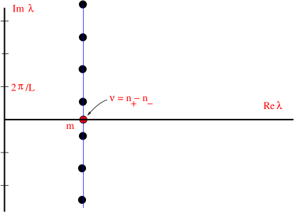
Figure 1: In the naive continuum picture, all eigenvalues of the Dirac operator lie along a line parallel to the imaginary axis. In a finite volume these eigenvalues become discrete. The real eigenvalues divide into distinct chiralities and define a topological invariant.

At zero chemical potential, all actions used in practice satisfy “$\gamma_{5}$ hermiticity”

$$\gamma_{5}D\gamma_{5}=D^{\dagger}.$$ (6)

With this condition all non-real eigenvalues occur in complex conjugate pairs, implying for the density

$$\rho(z)=\rho(z^{*}).$$ (7)

This property will be shared by all the operators considered in the following discussion.

The quest is to find general statements relating the behavior of the eigenvalue density to physical properties of the theory. I repeat the earlier warning; $\rho$ depends on the distribution of gauge fields $A$ which in turn is weighted by $\rho$ which depends on the distribution of $A$ ….

2.1 The continuum

Of course the continuum theory is only really defined as the limit of the lattice theory. Nevertheless, it is perhaps useful to recall the standard picture, where the Dirac operator

$$D=\gamma_{\mu}(\partial_{\mu}+igA_{\mu})+m$$

is the sum of an anti-hermitian piece and the quark mass $m$. All eigenvalues have the same real part $m$

$$\rho(x+iy)=\delta(x-m)\tilde{\rho}(y).$$

The eigenvalues lie along a line parallel to the imaginary axis, while the hermiticity condition of Eq. (6) implies they occur in complex conjugate pairs.

Restricted to the subspace of real eigenvalues, $\gamma_{5}$ commutes with $D$ and thus these eigenvectors can be separated by chirality. The difference between the number of positive and negative eigenvalues of $\gamma_{5}$ in this subspace defines an index related to the topological structure of the gauge fields.$\!{}^{{\bf?}}$ The basic structure is sketched in Fig. (1).

The Banks and Casher argument relates a non-vanishing $\tilde{\rho}(0)$ to the chiral condensate occurring when the mass goes to zero. I will say more on this later in the lattice context.

Note that the naive picture suggests a symmetry between positive and negative mass. Due to anomalies, this is spurious. With an odd number of flavors, the theory obtained by flipping the signs of all fermion masses is physically inequivalent to the initial theory.

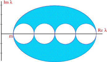
Figure 2: Free Wilson fermions display an eigenvalue spectrum with a momentum dependent real part. This removes doublers by giving them a large effective mass.

2.2 Wilson fermions

The lattice reveals that the true situation is considerably more intricate due to the chiral anomaly. Without ultraviolet infinities, all naive symmetries of the lattice action are true symmetries. Naive fermions cannot have anomalies, which are cancelled by extra states referred to as doublers. Wilson fermions$\!{}^{{\bf?}}$ avoid the this issue by giving a large real part to those eigenvalues corresponding to the doublers. For free Wilson fermions the eigenvalue structure displays a simple pattern as shown in Fig. (2).

As the gauge fields are turned on, this pattern will fuzz out. An additional complication is that the operator $D$ is no longer normal, i.e. $[D,D^{\dagger}]\neq 0$ and the eigenvectors need not be orthogonal. The complex eigenvalues are still paired, although, as the gauge fields vary, complex pairs of eigenvalues can collide and separate along the real axis. In general, the real eigenvalues will form a continuous distribution.

As in the continuum, an index can be defined from the spectrum of the Wilson-Dirac operator. Again, $\gamma_{5}$ hermiticity allows real eigenvalues to be sorted by chirality. To remove the contribution of the doubler eigenvalues, select a point inside the leftmost open circle of Fig. (2). Then define the index of the gauge field to be the net chirality of all real eigenvalues below that point. For smooth gauge fields this agrees with the topological winding number obtained from their interpolation to the continuum. It also corresponds to the winding number discussed below for the overlap operator.

2.3 The overlap

Wilson fermions have a rather complicated behavior under chiral transformations. The overlap formalism$\!{}^{{\bf?}}$ simplifies this by first projecting the Wilson matrix $D_{W}$ onto a unitary operator

$$V=(D_{W}D_{W}^{\dagger})^{-1/2}D_{W}.$$ (8)

This is to be understood in terms of going to a basis that diagonalizes $D_{W}D_{W}^{\dagger}$, doing the inversion, and then returning to the initial basis. In terms of this unitary quantity, the overlap matrix is

$$D=1+V.$$ (9)

The projection process is sketched in Fig. (3). The mass used in the starting Wilson operator is taken to a negative value so selected that the low momentum states are projected to low eigenvalues, while the doubler states are driven towards $\lambda\sim 2$.

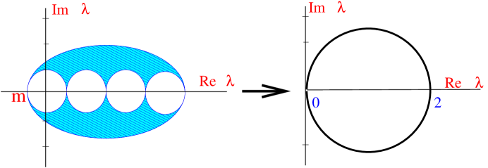
Figure 3: The overlap operator is constructed by projecting the Wilson Dirac operator onto a unitary operator.

The overlap operator has several nice properties. First, it satisfies the Ginsparg-Wilson relation,$\!{}^{{\bf?}}$ most succinctly written as the unitarity of $V$ coupled with its $\gamma_{5}$ hermiticity

$$\gamma_{5}V\gamma_{5}V=1.$$ (10)

As it is constructed from a unitary operator, normality of $D$ is guaranteed. But, most important, it exhibits a lattice version of an exact chiral symmetry.$\!{}^{{\bf?}}$ The fermionic action $\overline{\psi}D\psi$ is invariant under the transformation

$$\psi\rightarrow e^{i\theta\gamma_{5}}\psi$$ (11)

$$\overline{\psi}\rightarrow\overline{\psi}e^{i\theta\hat{\gamma}_{5}}$$ (12)

where

$$\hat{\gamma}_{5}=V\gamma_{5}.$$ (13)

As with $\gamma_{5}$, this quantity is Hermitean and its square is unity. Thus its eigenvalues are all plus or minus unity. The trace defines an index

$$\nu={1\over 2}{\rm Tr}\hat{\gamma}_{5}$$ (14)

which plays exactly the role of the index in the continuum.

It is important to note that the overlap operator is not unique. Its precise form depends on the particular initial operator chosen to project onto the unitary form. Using the Wilson-Dirac operator for this purpose, the result still depends on the input mass used. From its historical origins in the domain wall formalism, this quantity is sometimes called the “domain wall height.”

Because the overlap is not unique, an ambiguity can remain in determining the winding number of a given gauge configuration. Issues arise when $D_{W}D_{W}^{\dagger}$ is not invertible, and for a given gauge field this can occur at specific values of the projection point. This problem can be avoided for “smooth” gauge fields. Indeed, an “admissibility condition,” $\!{}^{{\bf?},{\bf?}}$ requiring all plaquette values to remain sufficiently close to the identity, removes the ambiguity. Unfortunately this condition is incompatible with reflection positivity.$\!{}^{{\bf?}}$ Because of these issues, it is not known if the topological susceptibility is in fact a well defined physical observable. On the other hand, as it is not clear how to measure the susceptibility in a scattering experiment, there seems to be little reason to care if it is an observable or not.

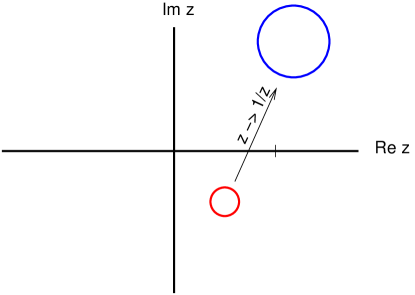
Figure 4: Inverting a complex circle generates another circle.

3 A Cheshire chiral condensate

Now that I have reviewed the basic framework, it is time for a little fun. I will calculate the chiral condensate in the overlap formalism. I should warn you that, in the interest of amusing you, I start the argument in an intentionally deceptive manner.

3.1 He’s here

I begin with the standard massless overlap theory. I want to calculate the quantity $\langle\overline{\psi}\psi\rangle$. Remarkably, this can be done exactly. I start with

$$\langle\overline{\psi}\psi\rangle=\langle{\rm Tr}D^{-1}\rangle=\left\langle\sum_{i}{1\over\lambda_{i}}\right\rangle=\left\langle\sum{\rm Re}{1\over\lambda_{i}}\right\rangle$$ (15)

where I have used the complex pairing of eigenvalues to cancel the imaginary parts. At the end, the average is to be taken over appropriately weighted gauge configurations.

Now the crucial feature of the overlap operator is that its eigenvalues all lie on a circle in the complex plane. An interesting property of a general complex circle is that the inverses of all its points generates another circle, as sketched in Fig. 4.

This process is, however, somewhat singular for the overlap operator itself since the corresponding circle touches the origin. In this case the inverted circle has infinite radius, i.e. it degenerates into a line. For the circle of the overlap operator, with center at $z=1$ and radius 1, the inverse circle is a line with real part 1/2 and parallel to the imaginary axis. This is sketched in Fig. 5.

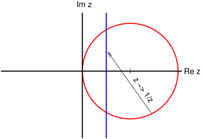
Figure 5: Inverting the overlap operator generates a line with real part 1/2.

This placement of eigenvalues enables an immediate calculation of the condensate

$$\langle\overline{\psi}\psi\rangle=\sum{\rm Re}{1\over\lambda_{i}}=\sum{1\over 2}={N\over 2}.$$ (16)

Here $N$ is the dimension of the matrix, and includes the expected volume factor.

So the condensate, supposedly a signal for spontaneous chiral symmetry breaking, does not vanish! But something is fishy, I didn’t use any dynamics. The result also is independent of gauge configuration.

3.2 He’s gone

So lets get more sophisticated. On the lattice, the chiral symmetry is more complicated than in the continuum, involving both $\gamma_{5}$ and $\hat{\gamma}_{5}$ in a rather intricate way. In particular, the operator $\overline{\psi}\psi$ does not transform in any simple manner under chiral rotations. A possibly nicer combination is $\overline{\psi}(1-D/2)\psi$. If I consider the rotation in Eq. (12) with $\theta=\pi/2$, this quantity becomes its negative. But it is also easy to calculate the expectation of this as well. The second term involves

$$\langle\overline{\psi}D\psi\rangle={\rm Tr}D^{-1}D={\rm Tr}I=N.$$ (17)

Putting the two pieces together

$$\langle\overline{\psi}(1-D/2)\psi\rangle=N/2-N/2=0.$$ (18)

So, I’ve lost the chiral condensate that I so easily showed didn’t vanish just a moment ago. Where did it go?

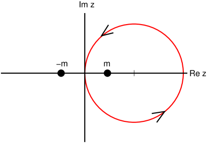
Figure 6: As the mass changes sign a pole moves between inside and outside the overlap circle. This generates a jump in the condensate.

3.3 He’s back

The issue lies in a careless treatment of limits. In finite volume, $\langle\overline{\psi}(1-D/2)\psi\rangle$ must vanish just from the exact lattice chiral symmetry. This vanishing occurs for all gauge configurations. To proceed, introduce a small mass and take the volume to infinity first and then the mass to zero. Toward this end, consider the quantity

$$\langle\overline{\psi}\psi\rangle=\sum_{i}{1\over\lambda_{i}+m}.$$ (19)

The signal for chiral symmetry breaking is a jump in this quantity as the mass passes through zero.

As the volume goes to infinity, replace the above sum with a contour integral around the overlap circle using $z=1+e^{i\theta}$. Up to the trivial volume factor, I should evaluate

$$i\int_{0}^{2\pi}d\theta{\rho(\theta)\over 1+e^{i\theta}+m}.$$ (20)

As the mass passes through zero, the pole at $z=-m$ passes between lying outside and inside the circle, as sketched in Fig. (6). As it passes through the circle, the residue of the pole is $\rho(0)=\lim_{\theta\rightarrow 0}\rho(\theta)$. Thus the integral jumps by $2\pi\rho(0)$. This is the overlap version of the Banks-Casher relation;$\!{}^{{\bf?}}$ a non-trivial jump in the condensate is correlated with a non-vanishing $\rho(0)$.

Note that the exact zero modes related to topology are supressed by the mass and do not contribute to this jump. For one flavor, however, the zero modes do give rise to a non-vanishing but smooth contribution to the condensate.$\!{}^{{\bf?}}$ More on this point later.

4 Another puzzle

For two flavors of light quarks one expects spontaneous symmetry breaking. This is the explanation for the light mass of the pion, which is an approximate Goldstone boson. In the above picture, the two flavor theory should have a non-vanishing $\rho(0)$.

Now consider the one flavor theory. In this case there should be no chiral symmetry. The famous $U(1)$ anomaly breaks the naive symmetry. No massless physical particles are expected when the quark mass vanishes. Furthermore, simple chiral Lagrangian arguments$\!{}^{{\bf?},{\bf?}}$ for multiple flavor theories indicate that no singularities are expected when just one of the quarks passes through zero mass. From the above discussion, this leads to the conclusion that for the one flavor theory $\rho(0)$ must vanish.

But now consider the original path integral after the fermions are integrated out. Changing the number of flavors $N_{f}$ manifests itself in the power of the determinant

$$\int dA\ |D|^{N_{f}}\ e^{-S_{g}(A)}.$$ (21)

Naively this suggests that as you increase the number of flavors, the density of low eigenvalues should decrease. But I have just argued that with two flavors $\rho(0)\neq 0$ but with one flavor $\rho(0)=0$. How can it be that increasing the number of flavors actually increases the density of small eigenvalues?

This is a clear example of how the non-linear nature of the problem can produce non-intuitive results. The eigenvalue density depends on the gauge field distribution, but the gauge field distribution depends on the eigenvalue density. It is not just the low eigenvalues that are relevant to the issue. Fermionic fields tend to smooth out gauge fields, and this process involves all scales. Smoother gauge fields in turn can give more low eigenvalues. Thus high eigenvalues influence the low ones, and this effect evidently can overcome the naive suppression from more powers of the determinant.

5 Æthereal instantons

Through the index theorem, the topological structure of the gauge field manifests itself in zero modes of the massless Dirac operator. Let me again insert a small mass and consider the path integral with the fermions integrated out

$$Z=\int dA\ e^{-S_{g}}\ \prod_{i}(\lambda_{i}+m).$$ (22)

If I take the mass to zero, any configurations which contain a zero eigenmode will have zero weight in the path integral. This suggests that for the massless theory, I can ignore any instanton effects since those configurations don’t contribute to the path integral.

What is wrong with this argument? The issue is not whether the zero modes contribute to the path integral, but whether they can contribute to physical correlation functions. To see how this goes, add some sources to the path integral

$$Z(\eta,\overline{\eta})=\int dA\ d\psi\ d\overline{\psi}\ e^{-S_{g}+\overline{\psi}(D+m)\psi+\overline{\psi}\eta+\overline{\eta}\psi}.$$ (23)

Differentiation (in the Grassmann sense) with respect to $\eta$ and $\overline{\eta}$ gives the fermionic correlation functions. Now integrate out the fermions

$$Z=\int dA\ e^{-S_{g}-\overline{\eta}(D+m)^{-1}\eta}\ \prod_{i}(\lambda_{i}+m).$$ (24)

If I consider a source that overlaps with one of the zero mode eigenvectors, i.e.

$$(\psi_{0},\eta)\neq 0,$$ (25)

the source contribution introduces a $1/m$ factor. This cancels the $m$ from the determinant, leaving a finite contribution as $m$ goes to zero.

With multiple flavors, the determinant will have a mass factor from each. When several masses are taken to zero together, one will need a similar factor from the sources for each. This product of source terms is the famous “‘t Hooft vertex.” $\!{}^{{\bf?}}$ While it is correct that instantons do drop out of $Z$, they survive in correlation functions.

While these issues are well understood theoretically, they can raise potential difficulties for numerical simulations. The usual numerical procedure generates gauge configurations weighted as in the partition function. For a small quark mass, topologically non-trivial configurations will be suppressed. But in these configurations, large correlations can appear due to instanton effects. This combination of small weights with large correlations can give rise to large statistical errors, thus complicating small mass extrapolations. The problem will be particularly severe for quantities dominated by anomaly effects, such as the $\eta^{\prime}$ mass. A possible strategy to alleviate this effect is to generate configurations with a modified weight, perhaps along the lines of multicanonical algorithms.$\!{}^{{\bf?}}$

Note that when only one quark mass goes to zero, the ’t Hooft vertex is a quadratic form in the fermion sources. This will give a finite but smooth contribution to the condensate $\langle\overline{\psi}\psi\rangle$. Indeed, this represents a non-perturbative additive shift to the quark mass. The size of this shift generally depends on scale and regulator details. Even with the Ginsparg-Wilson condition, the lattice Dirac operator is not unique, and there is no proof that two different forms have to give the same continuum limit for vanishing quark mass. Because of this, the concept of a single massless quark is not physical,$\!{}^{{\bf?}}$ invalidating one popular proposed solution to the strong CP problem. This ambiguity has been noted for heavy quarks in a more perturbative context$\!{}^{{\bf?}}$ and is often referred to as the “renormalon” problem. The issue is closely tied to the problems mentioned earlier in defining the topological susceptibility.

6 Summary

In short, thinking about the eigenvalues of the Dirac operator in the presence of gauge fields can give some insight, for example the elegant Banks-Casher picture for chiral symmetry breaking. Nevertheless, care is necessary because the problem is highly non-linear. This manifests itself in the non-intuitive example of how adding flavors enhances rather than suppresses low eigenvalues.

Issues involving zero mode suppression represent one facet of a set of connected unresolved issues. Are there non-perturbative ambiguities in quantities such as the topological susceptibility? How essential are rough gauge fields, i.e. gauge fields on which the winding number is ambiguous? How do these issues interplay with the quark masses? I hope the puzzles presented here will stimulate more thought along these lines.

References

References

- [1] T. Banks and A. Casher, Nucl. Phys. B 169 (1980) 103.
- [2] P. H. Ginsparg and K. G. Wilson, Phys. Rev. D 25 (1982) 2649.
- [3] H. Neuberger, Phys. Lett. B 417 (1998) 141 [arXiv:hep-lat/9707022].
- [4] Y. Aoki et al., Phys. Rev. D 69 (2004) 074504 [arXiv:hep-lat/0211023].
- [5] A. Duncan, E. Eichten and H. Thacker, Phys. Rev. D 59 (1999) 014505 [arXiv:hep-lat/9806020].
- [6] J. C. Osborn, K. Splittorff and J. J. M. Verbaarschot, Phys. Rev. Lett. 94 (2005) 202001 [arXiv:hep-th/0501210].
- [7] S. R. Coleman, in C77-07-23.7 HUTP-78/A004 Lecture delivered at 1977 Int. School of Subnuclear Physics, Erice, Italy, Jul 23-Aug 10, 1977.
- [8] K. G. Wilson, in New Phenomena In Subnuclear Physics. Part A. Proceedings of the First Half of the 1975 International School of Subnuclear Physics, Erice, Sicily, July 11 - August 1, 1975, ed. A. Zichichi, Plenum Press, New York, 1977, p. 69.
- [9] M. Luscher, Phys. Lett. B 428 (1998) 342 [arXiv:hep-lat/9802011].
- [10] M. Luscher, Commun. Math. Phys. 85 (1982) 39.
- [11] P. Hernandez, K. Jansen and M. Luscher, Nucl. Phys. B 552 (1999) 363 [arXiv:hep-lat/9808010].
- [12] M. Creutz, Phys. Rev. D 70 (2004) 091501 [arXiv:hep-lat/0409017].
- [13] P. H. Damgaard, Nucl. Phys. B 556 (1999) 327 [arXiv:hep-th/9903096].
- [14] P. Di Vecchia and G. Veneziano, Nucl. Phys. B 171 (1980) 253.
- [15] M. Creutz, Phys. Rev. Lett. 92, 201601 (2004) [arXiv:hep-lat/0312018].
- [16] G. ’t Hooft, Phys. Rev. Lett. 37 (1976) 8.
- [17] B. A. Berg and T. Neuhaus, Phys. Rev. Lett. 68 (1992) 9 [arXiv:hep-lat/9202004].
- [18] M. Creutz, Phys. Rev. Lett. 92 (2004) 162003.
- [19] I. I. Y. Bigi, M. A. Shifman, N. G. Uraltsev and A. I. Vainshtein, Phys. Rev. D 50 (1994) 2234 [arXiv:hep-ph/9402360].