SU(2) Gluodynamics and ${\mathrm{HP}^{1}}$ $\sigma$-model Embedding:
Scaling, Topology and Confinement

Abstract

We investigate recently proposed ${\mathrm{HP}^{1}}$ $\sigma$-model embedding method aimed to study the topology of SU(2) gauge fields. The ${\mathrm{HP}^{1}}$ based topological charge is shown to be fairly compatible with various known definitions. We study the corresponding topological susceptibility and estimate its value in the continuum limit. The geometrical clarity of ${\mathrm{HP}^{1}}$ approach allows to investigate non-perturbative aspects of SU(2) gauge theory on qualitatively new level. In particular, we obtain numerically precise estimation of gluon condensate and its leading quadratic correction. Furthermore, we present clear evidences that the string tension is to be associated with global (percolating) regions of sign-coherent topological charge. As a byproduct of our analysis we estimate the continuum value of quenched chiral condensate and the dimensionality of regions, which localize the lowest eigenmodes of overlap Dirac operator.

I Introduction

The topological aspects of gauge theories had always been the prime topic for the lattice community. However, the real breakthrough here is due to the construction of chirally symmetric overlap Dirac operator on the lattice Neuberger:1997fp , which via Atiyah-Singer index theorem Atiyah:1971rm applied in lattice settings overlap allowed to investigate the topology of equilibrium vacuum fields. Since then a lot of remarkable results were obtained, among which the discovery of global (percolating) regions of sign-coherent topological charge Horvath-structures ; Gubarev:2005rs is worth to be mentioned. Note that the overlap-based approach to the gauge fields topology is rather involved technically, however, the intricacy of the method is not the only problem here. What is more important for us is the factual absence of geometrically clean microscopic picture behind the topological fluctuations in the overlap approach, which is in a sharp contrast with what is known from seminal papers Atiyah:1978ri ; Drinfeld:1978xr about the topology of Yang-Mills fields (see also HPN-various ).

Recently the alternative definition of the topological charge Gubarev:2005rs has been put forward, which is based essentially on the same topological ideas as were used in Atiyah:1978ri ; Drinfeld:1978xr . The essence of the method consists in finding the nearest (in the configuration space) to given SU(2) gauge background configuration of scalar fields representing non-linear $\sigma$-model with target space being the quaternionic projective space ${\mathrm{HP}^{n}}$ (see Ref. Gubarev:2005rs for missing details). The relevance of ${\mathrm{HP}^{n}}$ spaces is by no means accidental, the close connection between $SU(2)$ Yang-Mills theory and ${\mathrm{HP}^{n}}$ $\sigma$-models is known for edges Atiyah:1978ri ; Drinfeld:1978xr ; HPN-various ; Dubrovin . Generically the idea is to realize the original $SU(2)$ gauge holonomy assigned to every lattice link as the non-Abelian geometrical phase factor associated with motion of scalar particle possessing non-trivial internal symmetry space. However, except for classical gauge backgrounds it is not possible to achieve this exactly, hence the appearance of the term ’nearest configuration’ above. Unfortunately, this is the weakest aspect of ${\mathrm{HP}^{n}}$ $\sigma$-model approach since the notion of nearest configuration could not, in fact, be conceived rigorously in the case of quantum fields and we have to rely mostly on the results of numerical simulations. However, we note that this is not a fatal restriction of the method, essentially the same problem exists, for instance, in overlap-based approach, where it was by no means evident a priori that chirally symmetric Dirac operator applied to thermalized fields is indeed local. Note that for equilibrium configurations the dependence upon the $\sigma$-model rank $n$ was found Gubarev:2005rs to be trivial  and for this reason we consider only the case $n=1$ below.

The crucial advantage of ${\mathrm{HP}^{1}}$ approach is its clean geometrical meaning, which not only allows to capture the gauge fields topology, but also permits the microscopic investigation of the topological fluctuations – the luxury which was not available so far. The prime purpose of the present publication is to put this assertion on numerically solid grounds. Note that some remarkable results we obtained already in Ref. Gubarev:2005rs and we by no means casting doubts on them. However, as far as the phenomenologically relevant quantities are concerned, the numerics should evidently be improved and we do this in present paper. In particular, after short theoretical introduction and description of the numerical algorithms (section II) we present in section III statistically convincing comparison of ${\mathrm{HP}^{1}}$ and overlap-based topological charges both measured on the same thermalized vacuum configurations. Furthermore, in section IV the scaling of ${\mathrm{HP}^{1}}$ based topological susceptibility with lattice spacing and volume is discussed in details and its rather unambiguous extrapolation to the continuum limit is presented. The outcome of this calculations makes us confident that ${\mathrm{HP}^{1}}$ topological charge is fairly compatible with overlap-based definition and is insensitive to lattice dislocations. Moreover, keeping in mind the technical complexity and geometrical obscurity of the overlap construction, we dare to claim that the ${\mathrm{HP}^{1}}$ $\sigma$-model embedding method is indeed advantageous both geometrically and computationally.

The geometrical explicitness of ${\mathrm{HP}^{1}}$ approach is crucial for the remaining part of our paper. Namely it allows us to investigate the topology related content of the original gauge fields in explicit manner by introducing the so called ${\mathrm{HP}^{1}}$ projection to be discussed in details in section V. Note that the term ’projection’ here has nothing in common with its nowadays conventional meaning, nevertheless we use it mostly due to the historical reasons. The results we obtain this way are indeed remarkable, however, before mentioning them we would like note the following. In this paper we intentionally leave aside any serious attempts to interpret the experimental data. In fact, the theoretical interpretation could indeed be given, moreover, it overlaps partially with moderns trends in the literature Gubarev:2005jm ; Polikarpov:2005ey ; A2 ; A2-review ; viz ; viz2 . However, consideration of the theoretical implications would leads us to quite lengthy discussions and for that reason we decided to focus exclusively on the experimental side of the problem. Our theoretical interpretation of the results presented here is to be published elsewhere future .

Section V is devoted to the investigation of the dynamics of ${\mathrm{HP}^{1}}$ projected fields obtained from vacuum configurations at various lattice spacings. We start in section V.1 from the consideration of the curvature of projected fields, which turns out to be extremely small. Furthermore, its spacing dependence does not contain any sign whatsoever of the perturbation theory contribution. Instead, the curvature vanishes in the limit $a\to 0$, the leading spacing corrections being quartic and quadratic in $a$. In turn, these leading terms are to be interpreted as the gluon condensate and quadratic power correction to it, for both of which we obtain numerically precise estimations and compare them with available literature. Then in section V.2 the confining properties of ${\mathrm{HP}^{1}}$ projected fields are investigated from various viewpoints. The conclusion is that these fields are indeed confining, moreover, the corresponding string tension accounts for the full $SU(2)$ string tension in the continuum limit. The geometrical clarity of the ${\mathrm{HP}^{1}}$ approach allows us to investigate in section V.2.2 the microscopic origin of the projected string tension. We present clear evidences that the string tension is to be associated with global (percolating) regions of sign-coherent topological charge mentioned above. Finally, to conclude the study of ${\mathrm{HP}^{1}}$ projected fields dynamics we consider in section V.3 the low lying spectrum of overlap Dirac operator in the projected background and show that both the spectral density and the localization properties of low lying modes are essentially the same as they are on the original fields. The quenched chiral condensate and the dimensionality of localization regions as they are seen within ${\mathrm{HP}^{1}}$ projection are estimated.

The results of section V could only be convincing provided that we make sure that the gauge fields components not surviving ${\mathrm{HP}^{1}}$ projection do not contribute to neither of non-perturbative observables discussed above. The problem is non-trivial due to the explicit gauge covariance of ${\mathrm{HP}^{1}}$ projection, however we believe that it is addressed adequately in section VI, where we show that this part of the original gauge fields could be defined unambiguously. Then it is the matter of straightforward calculation to show that the correspondingly constructed configurations are:

i) topologically trivial, in a sense that the topological charge in both ${\mathrm{HP}^{1}}$ and overlap definitions vanishes identically on all configurations we have in our disposal;

ii) deconfining, the string tension vanishes while the heavy quark potential is still compatible with Coulomb law;

iii) trivial from the fermionic viewpoint, the low lying spectrum of the Dirac operator disappears completely, we were unable to find even a single low lying eigenmode on all our configurations.

These findings are the most stringent evidences that what had been left aside by ${\mathrm{HP}^{1}}$ projection corresponds to pure perturbation theory. At the same time, they show that the results and estimations of various non-perturbative observables, which were obtained in section V, are indeed reliable. Keeping in mind that the actual numbers are in complete agreement with the existing literature, we dare to claim that the ${\mathrm{HP}^{1}}$ projection is, in fact, the unique method allowing to achieve numerically most accurate results.

Finally, let us mention that the approach developed in sections V, VI is parallel in spirit to what is known in the literature as ’vortex removal’ vortex-removal and ’monopole removal’ Bornyakov:2005wp procedures. However, we stress that the ${\mathrm{HP}^{1}}$ projection is by no means similar to them both physically and technically.

II Theoretical Background and Numerical Algorithms

In this section we briefly outline the recent approach Gubarev:2005rs aimed to investigate $SU(2)$ gauge fields topology. This material is included to introduce the necessary notations and to make the paper self-contained (for details and further references see Gubarev:2005rs ). In particular, in this section we precisely describe the numerical methods utilized in our paper. Note that the present numerical implementation is slightly different from that of Gubarev:2005rs although we checked that the difference is completely inessential physics-wise.

Quaternionic projective space ${\mathrm{HP}^{1}}$ can be viewed as the factor space ${\mathrm{HP}^{1}}=S^{4}=S^{7}/S^{3}$ (second Hopf fibering) and its lowest non-trivial homotopic group is $\pi_{4}({\mathrm{HP}^{1}})=\pi_{3}(S^{3})=Z$. The simplest explicit parametrization of ${\mathrm{HP}^{1}}$ is provided by normalized quaternionic vectors

$$|\,q\,\rangle=[q_{0},q_{1}]^{T}\,,\quad q_{i}\in\mathrm{H}\,,\quad\langle\,q\,|\,q\,\rangle=\bar{q}_{i}q_{i}=1\in\mathrm{H}\,,$$ (1)

where $[...]^{T}$ indicates transposition, $\mathrm{H}$ is the field of real quaternions, $q_{i}=q_{i}^{\alpha}e_{\alpha}\in\mathrm{H}$, $\alpha=0,...,3$ and $e_{\alpha}$ are the quaternionic units

$$e_{0}=1\,,\quad e_{i}e_{j}=-\delta_{ij}-\varepsilon_{ijk}e_{k}\,,\,\,\,\,i,j,k=1,2,3$$ (2)

with conjugation defined as usual

$$\bar{q}_{i}=q_{i}^{\alpha}\bar{e}_{\alpha}\,,\qquad\bar{e}_{0}=e_{0}\,,\,\,\,\,\bar{e}_{i}=-e_{i}\,,\,\,\,\,i=1,2,3\,.$$ (3)

The states $|\,q\,\rangle$ describe $7$-dimensional sphere, $|\,q\,\rangle\in S^{7}$, while the ${\mathrm{HP}^{1}}$ space is the set of equivalence classes of $|\,q\,\rangle$ with respect to the right multiplication by unit quaternions (elements of SU(2) group)

$$|\,q\,\rangle\sim|\,q\,\rangle\,\upsilon\,,\qquad|\upsilon|^{2}\equiv\bar{\upsilon}\upsilon=1\,,\quad\upsilon\in\mathrm{H}\,.$$ (4)

The gauge invariance (4) allows to introduce almost everywhere inhomogeneous coordinate $\omega=q_{1}q^{-1}_{0}=y^{\alpha}e_{\alpha}\in\mathrm{H}$ on ${\mathrm{HP}^{1}}$ space

$$|\,q\,\rangle=[q_{0},q_{1}]^{T}~{}\sim~{}\frac{1}{\sqrt{1+|\omega|^{2}}}\,[1,\omega]^{T}\,.$$ (5)

The alternative parametrization is provided by 5-dimensional unit vector $n^{A}$, $A=0,...,4$ defined by

$$n^{A}=\langle\,q\,|\gamma^{A}|\,q\,\rangle\,,$$ (6)

where $\gamma^{A}$ are five Euclidean Dirac matrices $\{\gamma^{\alpha},\gamma^{5}\}$ viewed as $2\times 2$ quaternionic ones. One could show that (6) is equivalent to the standard stereographic projection which relates $n^{A}$ with inhomogeneous coordinate $\omega=y^{\alpha}e_{\alpha}$ above

$$n^{\alpha}=\frac{2y^{\alpha}}{1+y^{2}}\,,\,\,\,\,\alpha=0,...,3\,,\qquad n^{4}=\frac{1-y^{2}}{1+y^{2}}\,.$$ (7)

It is clear that non-linear $\sigma$-model with target space ${\mathrm{HP}^{1}}$ would be non-trivial provided that the base space is taken to be 4-sphere $S^{4}$. The corresponding topological charge

$$Q=\frac{1}{(8\pi)^{2}}\int d^{4}x\,\,\varepsilon^{\mu\nu\lambda\rho}\,\varepsilon_{ABCDE}\cdot~{}~{}~{}~{}~{}~{}~{}~{}~{}~{}~{}~{}~{}~{}~{}~{}~{}~{}~{}$$ (8)

$$~{}~{}~{}~{}~{}~{}~{}~{}~{}~{}~{}~{}~{}~{}~{}~{}~{}~{}~{}\cdot n^{A}\partial_{\mu}n^{B}\partial_{\nu}n^{C}\partial_{\lambda}n^{D}\partial_{\rho}n^{E}$$

is geometrically the sum of oriented infinitesimal volumes in the image of $n^{A}(x):S^{4}\to{\mathrm{HP}^{1}}$.

As usual it is convenient to introduce auxiliary SU(2) gauge fields

$$A_{\mu}=-A^{\dagger}_{\mu}=-\langle\,q\,|\partial_{\mu}|\,q\,\rangle\,,$$ (9)

transforming as $A_{\mu}\to\bar{\upsilon}A_{\mu}\upsilon-\bar{\upsilon}\partial_{\mu}\upsilon$ under (4). Then the topological charge (8) is expressible solely in terms of $A_{\mu}$

$$Q=\frac{1}{32\pi^{2}}\int d^{4}x\,\,\varepsilon^{\mu\nu\lambda\rho}\,\,\mathrm{Tr}\,F_{\mu\nu}F_{\lambda\rho}\,,$$ (10)

$$F_{\mu\nu}=\partial_{\mu}A_{\nu}-\partial_{\nu}A_{\mu}+[A_{\mu},A_{\nu}]\,,$$

being essentially equivalent to the familiar topological charge of the gauge fields (9). Note that Eq. (10) is by no means accidental, the deep connection between ${\mathrm{HP}^{n}}$ $\sigma$-models and SU(2) Yang-Mills theory is known for edges (see, e.g., Refs. Atiyah:1978ri ; Drinfeld:1978xr ; HPN-various ; Dubrovin ). In particular, the geometry of gauge fields could best be analyzed in the ${\mathrm{HP}^{n}}$ $\sigma$-models context. In fact, all known instantonic solutions of Yang-Mills theory could be considered as induced by the topological configurations of suitable ${\mathrm{HP}^{n}}$ $\sigma$-models.

As is discussed in length in Ref. Gubarev:2005rs , it is natural to expect that the construction of nearest (in the configuration space) to the given gauge background ${\mathrm{HP}^{n}}$ fields captures accurately the gauge fields topology leaving aside the non-topological properties of the background. Note that for classical gauge fields the corresponding ${\mathrm{HP}^{n}}$ $\sigma$-model reproducing Eq. (9) is known to be unique HPN-various . However, the mathematical rigour is lost in case of ’hot’ vacuum configurations and we could only hope to find the nearest in the sense of Eq. (9) $\sigma$-model fields. The proposition of Ref. Gubarev:2005rs was to minimize the functional

$$F(A,q)~{}=~{}\int\left(A_{\mu}~{}+~{}\langle\,q\,|\partial_{\mu}|\,q\,\rangle\right)^{2}$$ (11)

for given $A_{\mu}$ with respect to all possible configurations of $|\,q_{x}\,\rangle$. On the lattice this equation translates into

$$F(U,q)~{}=~{}1-\frac{1}{4V}\sum\limits_{x,\mu}\mathrm{Sc}\left[\frac{\langle\,q_{x}\,|\,q_{x+\mu}\,\rangle}{|\langle\,q_{x}\,|\,q_{x+\mu}\,\rangle|}\,U^{\dagger}_{x,\mu}\right]\,,$$ (12)

where lattice gauge fields are denoted by $U_{x,\mu}\in SU(2)$, $V$ is the lattice volume and quaternionic scalar part is $\mathrm{Sc}[q]=(q+\bar{q})/2$. The configuration $|\,q_{x}\,\rangle$ which provides the minimum to $F(U,q)$ is the best possible ${\mathrm{HP}^{n}}$ fields approximation to the original gauge potentials

$$U_{x,\mu}~{}\approx~{}U^{\mathrm{HP}}_{x,\mu}~{}\equiv~{}\frac{\langle\,q_{x}\,|\,q_{x+\mu}\,\rangle}{|\langle\,q_{x}\,|\,q_{x+\mu}\,\rangle|}\,,$$ (13)

while the minimum value of (12) is a natural measure of the approximation quality. Furthermore, it was shown in Ref. Gubarev:2005rs that for equilibrium gauge configurations the dependence on the $\sigma$-model rank $n$ is trivial since the quality of the approximation (13) does not depend on $n$. Therefore, it seems to be legitimate to consider solely the case $n=1$ and only ${\mathrm{HP}^{1}}$ $\sigma$-model embedding is investigated below. Note that usually the extremization tasks like (12), (13) are expected to be plagued by Gribov copies problem. However, basing on the results of Ref. Gubarev:2005rs we assert that this issue is most likely irrelevant. Additional indirect evidence is provided by the fact that we changed slightly the extremization algorithm (see below) compared to that of Ref. Gubarev:2005rs , however, all physically relevant results turned out to be the same. As far as the actual numerical algorithms used in this paper are concerned, they could be summarized as follows.

• ${\mathrm{HP}^{1}}$ $\sigma$-model embedding.

The functional (12) was minimized sequentially at each lattice site, the non-linearity was taken into account by performing 3 iterations

$$|\,q^{(i+1)}_{x}\,\rangle\propto\sum\limits_{\mu}\left[\frac{|\,q_{x+\mu}\,\rangle U^{\dagger}_{x,\mu}}{|\langle\,q^{(i)}_{x}\,|\,q_{x+\mu}\,\rangle|}+\frac{|\,q_{x-\mu}\,\rangle U_{x-\mu,\mu}}{|\langle\,q^{(i)}_{x}\,|\,q_{x-\mu}\,\rangle|}\right]$$ (14)

at each point $x$ and then sweeping number of times through all the lattice until the algorithm converges. The proportionality factor, which is omitted in (14), is chosen to ensure the normalization condition $\langle\,q^{(i)}_{x}\,|\,q^{(i)}_{x}\,\rangle=1$ at each iteration. The stopping criterion was that the distance between old and new $|\,q\,\rangle$ values at all lattice sites in between two consecutive sweeps is smaller than $10^{-4}$

$$\max\limits_{x}\,(1~{}-~{}|\langle\,q^{old}_{x}\,|\,q^{new}_{x}\,\rangle|^{2})~{}<~{}10^{-4}\,.$$ (15)

Note that the value of r.h.s. is the result of trade-off between the computational demands and the needed numerical accuracy (see below). It turns out that Eq. (15) provides the accuracy of $\min_{q}F(U,q)$ calculation of order $10^{-6}$ which is the same as was used in Gubarev:2005rs . As far as the Gribov copies problem is concerned, we always considered 10 random initial distributions $|\,q_{x}\,\rangle$ and then selected the best minimum found.

• Global topological charge and topological density.

The topological charge density in terms of the ${\mathrm{HP}^{1}}$ $\sigma$-model fields is given by the oriented 4-volumes of spherical tetrahedra $T$ embedded into ${\mathrm{HP}^{1}}=S^{4}$ (image of $n^{A}:S^{4}\to{\mathrm{HP}^{1}}$). Unfortunately, the only way to estimate these volumes is to use the Monte Carlo technique which however forbids the exact volume evaluation. In this paper we used precisely the same algorithm of topological charge density calculation which was discussed in length in Gubarev:2005rs . In particular, the embedded ${\mathrm{HP}^{1}}$ $\sigma$-model assigns 5 unit five-dimensional vectors $n^{A}_{{i}}$ $i=0,...,4$ to every simplex ${\cal T}$ of physical space triangulation and the topological charge density in simplex ${\cal T}$ is given by

$$q({\cal T})=\frac{3}{8\pi^{2}}\,\mathrm{sign}\left(\mathrm{det}_{iA}\,[n^{A}_{(i)}]\right)\cdot V(T)\,,$$ (16)

where $V(T)$ is the volume of spherical tetrahedron $T$ and normalization factor $8\pi^{2}/3$ is the total volume of $S^{4}$. The corresponding topological charge

$$Q_{float}=\sum\limits_{\cal T}q({\cal T})$$ (17)

is not integer valued due to finite accuracy of Monte Carlo estimation of $V(T)$. However, for high enough accuracy of calculation at each simplex the non-integer valuedness of the topological charge is in fact irrelevant and we could safely identify

$$Q=\left[\,Q_{float}\,\right]\,,$$ (18)

where $[x]$ denotes the nearest to $x$ integer number. The validity of the identification (18) was discussed in details in Gubarev:2005rs . Here we note that there exist an additional cross-check of Eq. (18) based on the observation that in order to get the global topological charge it is not necessary to calculate its density in the bulk. It is sufficient to count (with sign) how many times a particular point $n_{0}\in{\mathrm{HP}^{1}}$ is covered by the image of $n^{A}:S^{4}\to{\mathrm{HP}^{1}}$

$$Q=\sum\limits_{\cal T}\,\left\{\begin{array}[]{cc}\mathrm{sign}\,\mathrm{det}_{iA}\,[n^{A}_{(i)}]&\mathrm{if}~{}~{}~{}n_{0}\in T\\ 0&\mathrm{otherwise}\end{array}\right.\,.$$ (19)

Evidently, Eq. (19) is computationally superior to (18) and we used it in present paper to calculate the topological charge. Moreover, the comparison of (18) and (19) provides the stringent calibration of Monte Carlo topological charge density evaluation (16). It goes without saying that we indeed checked that both definitions (18), (19) give exactly the same topological charge on all available configurations. Finally, we remark that slicing of hypercubical lattice into simplices was done according to Kronfeld:1986ts .

$\beta$ $a$,fm $L_{t}$ $L_{s}$ $V^{phys},\mathrm{fm}^{4}$ $N^{conf}$ $N^{conf}_{q}$ Fixed Volume 2.3493 0.1397(15) 10 10 3.8(2) 300 - 2.3772 0.1284(15) 14 10 3.8(2) 300 - 2.3877 0.1242(15) 16 10 3.8(2) 300 - 2.4071 0.1164(15) 12 12 3.8(2) 200 - 2.4180 0.1120(15) 14 12 3.8(2) 100 - 2.4273 0.1083(15) 16 12 3.8(2) 250 - 2.4500 0.0996(22) 14 14 3.8(2) 200 - 2.5000 0.0854(4) 18 16 3.92(7) 200 - Fixed Spacing 2.4180 0.1120(15) 14 14 6.0(3) 200 - 2.4180 0.1120(15) 16 16 10.3(6) 200 - 2.4180 0.1120(15) 18 18 16.5(9) 200 - 2.4000 0.1193(9) 16 16 13.3(4) 198 - 2.4750 0.0913(6) 16 16 4.6(1) 380 40 2.6000 0.0601(3) 28 28 8.0(2) 50 -

Table 1: Simulation parameters.

• Simulation parameters.

Our numerical measurements were performed on 14 sets (Table 1) of statistically independent SU(2) gauge configurations generated with standard Wilson action. The data sets are subdivided naturally into three groups indicated in Table 1. The fixed volume configurations are exactly the same as ones used in Refs. Gubarev:2005jm ; Polikarpov:2005ey in studying low lying Dirac eigenmodes localization properties. This allows us to make statistically significant comparison of ${\mathrm{HP}^{1}}$ $\sigma$-model approach and the overlap-based topological charge definition (section III). Gauge configurations at fixed spacing were generated to investigate the finite volume dependence of ${\mathrm{HP}^{1}}$-based topological susceptibility (section IV). In addition to the gauge configurations at $\beta=2.400$, $2.475$ which were analyzed already in Ref. Gubarev:2005rs , we also include the data set at $\beta=2.600$ with finest lattice spacing we have so far.

The last column in Table 1 represents the number of configurations on which we calculated the bulk topological charge density using the above described algorithm. Note that it is slightly different from that of Ref. Gubarev:2005rs and this explains the relatively small number of analyzed configurations. We stress that the results obtained with modified method remain essentially the same. Nevertheless, for honesty reasons the old data is not included in the present study. The relatively small number of configurations on which we calculated the bulk topological density distribution does not spoil the statistical significance of our results. Indeed, the majority of observables to be discussed below depend only upon the global topological charge obtained via Eq. (19) and upon the corresponding ${\mathrm{HP}^{1}}$ $\sigma$-model. In turn the ${\mathrm{HP}^{1}}$ fields were constructed for all configurations listed in Table 1 thus ensuring the statistical significance of our results.

The lattice spacing values quoted in Table 1 were partially taken from Refs. Lucini:2001ej ; spacings and fixed by the physical value of SU(2) string tension $\sqrt{\sigma}=440~{}\mathrm{MeV}$. Note that not all $\beta$-values listed in Table 1 could be found in the literature. In this case the lattice spacings and corresponding rather conservative error estimates were obtained via interpolation in between the points quoted in Lucini:2001ej ; spacings .

III ${\mathrm{HP}^{1}}$-based Topological Charge of Semiclassical and Vacuum Fields

The validity of ${\mathrm{HP}^{1}}$-based topological charge definition could only be convincing provided that we confront it with other known topological charge constructions. The preliminary study of this problem was already undertaken in Ref. Gubarev:2005rs , however, only correlation of local topological densities in ${\mathrm{HP}^{1}}$ and overlap-based approaches on relatively small statistics was considered in that paper. Here we fill this gap and compare the distribution of the ${\mathrm{HP}^{1}}$ global topological charge $Q_{HP^{1}}$, Eq. (19), with that in field-theoretical DiVecchia:1981qi and overlap-based Neuberger:1997fp ; overlap constructions.

Before presenting the results of our measurements let us discuss what could be the proper quantitative characteristic of the correlation between various definitions of lattice topological charge. The problem is that there is no commonly accepted viewpoint in the literature, usually people just consider the cumulative distribution of the topological charge in pair of definitions. For instance, in Ref. Cundy:2002hv the topological charge distribution histogram in the plane  $(Q_{clover},Q_{overlap})$ was presented, however, no quantitative measure of correlation between $Q_{clover}$ and $Q_{overlap}$ was given. Below we discuss two observables which quantify the notion of correlation between the topological charges $Q_{i}$ and $Q_{j}$ obtained via some abstract constructions “i” and “j” correspondingly. The first one could be obtained from the above mentioned cumulative distribution in $(Q_{i},Q_{j})$ plane by noting that the complete equivalence of “i” and “j” constructions would give $Q_{i}=Q_{j}$ identically and therefore the entire plot would collapse into $Q_{i}=Q_{j}$ line. On the other hand, any disagreement of “i” and “j” approaches would make the cumulative histogram broader and therefore it is natural to consider the ratio of the widths of cumulative distribution projected onto the lines $Q_{i}=-Q_{j}$ and $Q_{i}=Q_{j}$, for which the limiting values are $0$ (exact equivalence of “i” and “j” constructions) and $\approx 1$ (no correlation of $Q_{i}$ and $Q_{j}$). Moreover, it is similar to what had been done in Cundy:2002hv thus allowing to compare our results with the existing literature. However, it is clear that the widths ratio is mostly graphical characteristic since the distribution along $Q_{i}=-Q_{j}$ line is not guaranteed to be Gaussian-like, hence the corresponding width is ambiguous in general. To ameliorate this we propose to consider the correlator

$$\eta^{i}_{j}~{}=~{}\frac{\langle Q_{i}\,Q_{j}\rangle}{\sqrt{\langle Q^{2}_{i}\rangle\,\langle Q^{2}_{j}\rangle}}\,,$$ (20)

where averages are to be taken on the same set of configurations. Note that the normalization in (20) is such that $\eta^{i}_{j}\approx 1$ for essentially equivalent “i” and “j” constructions, while $\eta^{i}_{j}=0$ in the case of complete decorrelation of $Q_{i}$ and $Q_{j}$.

With all these preliminaries, let us compare our approach with field-theoretical method, which in turn could be applied reliably only on semiclassical (cooled) configurations. Thus its comparison with $Q_{{\mathrm{HP}^{1}}}$ is rather technical issue related mostly to the validity of $Q_{{\mathrm{HP}^{1}}}$ construction on semiclassical background. To this end we generated 300 cooled configurations (not included into Table 1) initially thermalized at $\beta=2.400$ on $16^{4}$ lattice. The cooling algorithm employed in our study is analogous to one described in GarciaPerez:1998ru . The original fields were cooled until the action stabilizes indicating that semiclassical regime had been reached. At this point we applied the algorithm of ${\mathrm{HP}^{1}}$ $\sigma$-model embedding thus obtaining $Q_{{\mathrm{HP}^{1}}}$ and simultaneously measured the field-theoretical topological charge $Q_{clover}$ defined by

$$Q_{clover}=\sum\limits_{x}q_{clover}(x)\,,$$ (21)

$$q_{clover}(x)=\frac{1}{32\pi^{2}}\varepsilon_{\mu\nu\lambda\rho}\mathop{\rm Tr}[\,F_{\mu\nu}(x)\,F_{\lambda\rho}(x)\,]\,,$$

where $F_{\mu\nu}$ is the $O(a^{4})$ improved lattice field-strength tensor Bilson-Thompson:2002jk ; deForcrand:1997sq . The resulting cumulative distribution of $Q_{\mathrm{HP}^{1}}$ and $Q_{clover}$ is presented on Fig. 1. As is evident from that figure both definitions are fairly compatible with each other making us confident that $Q_{\mathrm{HP}^{1}}$ and $Q_{clover}$ identify essentially the same topology on all considered data sets. The disagreement between $Q_{\mathrm{HP}^{1}}$ and $Q_{clover}$ is only seen in a few points which, however, is to be expected (see Ref. Cundy:2002hv for discussion of this issue in case of field-theoretical and overlap constructions). For this reason the above discussed widths ratio is certainly very small and is comparable with zero within the statistical errors. As far as the correlator (20) is concerned, its numerical value is

$$\eta^{clover}_{\mathrm{HP}^{1}}~{}=~{}0.94(1)$$ (22)

and indeed is very close to unity.

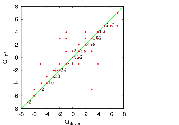
Figure 1: Cumulative distribution of $Q_{\mathrm{HP}^{1}}$, Eq. (19) and $Q_{clover}$, Eq. (21), on 300 cooled configurations initially thermalized at $\beta=2.400$ on $16^{4}$ lattice.

Turn now to the most interesting comparison of ${\mathrm{HP}^{1}}$ topological charge with becoming standard now construction based on Atiyah-Singer index theorem applied to chirally symmetric overlap Dirac operator Neuberger:1997fp ; overlap . Explicitly the overlap operator is given by

$$D=\frac{\rho}{a}\left(1+\frac{A}{\sqrt{AA^{\dagger}}}\right),\,\quad A=D_{W}-\frac{\rho}{a},$$ (23)

where $A$ is the Wilson Dirac operator with negative mass term and we used the optimal value $1.4$ of $\rho$ parameter. Anti-periodic (periodic) boundary conditions in time (space) directions were employed. To compute the sign function $\mathop{\rm sign}(A)=A/\sqrt{AA^{\dagger}}\equiv\gamma_{5}\mathop{\rm sign}(H)$, where $H=\gamma_{5}A$ is hermitian Wilson Dirac operator, we used the minmax polynomial approximation Giusti:2002sm . In order to improve the accuracy and performance about 50 lowest eigenmodes of $H$ were projected out. Note that the eigenvalues of $D$ are distributed on the circle of radius $\rho$ centered at $(\rho,0)$ in the complex plane. Below we will need to relate them with continuous eigenvalues of the Dirac operator and therefore the circle was stereographically projected onto the imaginary axis zenkin ; Capitani:1999uz .

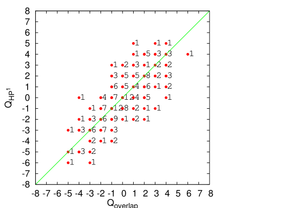
Figure 2: Cumulative distribution of $Q_{\mathrm{HP}^{1}}$, Eq. (19) and $Q_{overlap}$, Eq. (24), on 200 fixed volume configurations at $\beta=2.500$, Table 1.

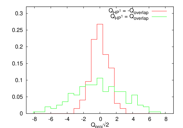
Figure 3: Projection of the cumulative distribution of $Q_{\mathrm{HP}^{1}}$ and $Q_{overlap}$ at $\beta=2.500$ onto the lines $Q_{\mathrm{HP}^{1}}=\pm Q_{overlap}$, along which $Q_{proj}\,\sqrt{2}$ is the corresponding integer valued coordinate. Note that both histograms are normalized separately.

It is well known that the knowledge of the spectrum of (23) allows to define the topological charge via Atiyah-Singer index theorem Atiyah:1971rm applied in lattice settings overlap

$$Q_{overlap}~{}=~{}n_{+}~{}-~{}n_{-}\,,$$ (24)

where $n_{+}$ $(n_{-})$ is the number of positive (negative) chirality zero eigenmodes. In order to compare $Q_{\mathrm{HP}^{1}}$ and $Q_{overlap}$ we considered both the cumulative distribution and the quantity (20) on $200+200$ fixed volume configurations at $\beta=2.450$ and $\beta=2.500$ (see Table 1). Note that since the width of $Q$ distribution is generically spacing dependent it would be unwise to mix $Q_{\mathrm{HP}^{1}}$, $Q_{overlap}$ cumulative distributions at different $\beta$-values and we present on Fig. 2 only $\beta=2.500$ results. Evidently both definitions are strongly correlated with each other although the distribution is notably broader than that on Fig. 1. The relative broadness of $Q_{\mathrm{HP}^{1}}$, $Q_{overlap}$ distribution is not surprising by itself, clearly it must be broader than that on cooled configurations. What is relevant here is its projection onto the lines $Q_{\mathrm{HP}^{1}}=\pm Q_{overlap}$ and the ratio of corresponding widths. The projected histograms are presented on Fig. 3, from which it is clear that they both are Gaussian-like, the widths ratio being about $1/3\div 1/4$. To get the feeling of the numbers involved it is instructive to remind the results of Ref. Cundy:2002hv , where the cumulative distribution of $Q_{clover}$ and $Q_{overlap}$ was considered. Note that the relevant plot of that paper refers to cooled configurations and its direct comparison with Figs. 2, 3 would be unfair since for cooled configurations the distribution is generically expected to be even narrower. However, it is pleasant to notice that the ratio of the corresponding widths in $Q_{clover}$, $Q_{overlap}$ distribution, which could be extracted from Ref. Cundy:2002hv , is larger than that of $Q_{\mathrm{HP}^{1}}$, $Q_{overlap}$ and is of order $1/3\div 1/2$. Thus we conclude that $Q_{\mathrm{HP}^{1}}$, $Q_{overlap}$ correlation seems to be even stronger than it is in the case of $Q_{clover}$ and $Q_{overlap}$ charges. Moreover, the strong correlation of $Q_{\mathrm{HP}^{1}}$ and $Q_{overlap}$ is also confirmed by the quantity (20) and what is probably more important is that it is rising with diminishing spacing

$$\eta^{overlap}_{\mathrm{HP}^{1}}(\beta=2.450)~{}=~{}0.71(1)\,,$$

$$\eta^{overlap}_{\mathrm{HP}^{1}}(\beta=2.500)~{}=~{}0.77(1)\,.$$

Note however that unlike the previous case of widths ratio the numerical values of $\eta^{overlap}_{\mathrm{HP}^{1}}$ cannot be compared with the existing literature.

To summarize, we found clear and statistically significant evidences that the construction of the topological charge based on ${\mathrm{HP}^{1}}$ $\sigma$-model embedding is fairly compatible with field-theoretical definition in case of semiclassical configurations and is strongly correlated with overlap-based approach in the case of equilibrium vacuum fields. In the next section we put the ${\mathrm{HP}^{1}}$ method under other tests, namely, consider the scaling properties of topological susceptibility defined via ${\mathrm{HP}^{1}}$ $\sigma$-model embedding.

IV Scaling of Topological Susceptibility

The basic topology related observable in pure Yang-Mills theory is the topological susceptibility which is formally defined as

$$\chi~{}=~{}\int d^{4}x\langle q(0)q(x)\rangle\,.$$ (25)

Here $q(x)$ is the topological charge density which is equal to $q_{clover}(x)$, Eq. (21), in the naive continuum limit. The topological susceptibility, being the quantity of prime phenomenological importance, is, in fact, not well defined within the definition (25) and is written usually as

$$\chi~{}=~{}\lim\limits_{\stackrel{{\scriptstyle a\to 0}}{{\scriptscriptstyle{V\to\infty}}}}\,\langle Q^{2}\rangle/V$$ (26)

in the context of lattice regularization, where $a$ and $V$ are the lattice spacing and lattice volume respectively. The purpose of this section is to study the limit (26) and obtain the estimate of the topological susceptibility in the continuum using the ${\mathrm{HP}^{1}}$ definition of the topological charge $Q\equiv Q_{\mathrm{HP}^{1}}$.

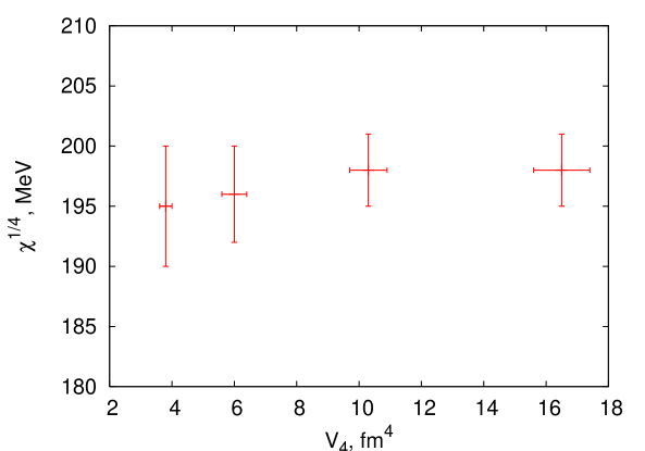
Figure 4: The topological susceptibility as a function of lattice volume both being expressed in physical units (fixed spacing configurations at $\beta=2.4180$, Table 1).

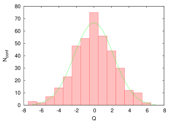
Figure 5: Topological charge distribution obtained at $\beta=2.475$ on $16^{4}$ lattices (380 configurations). Curve represents the best fit to Eq. (27).

Due to the absence of massless excitations in pure glue theory the topological susceptibility is expected to reach its infinite volume limit exponentially fast with increasing lattice size. The characteristic length of exponential fall off is dictated by lightest glueball mass $(1.5\mathrm{~{}GeV})^{-1}\approx 0.15\mathrm{~{}fm}$ and therefore we expect that finite-volume effects are negligible for our lattices. To confirm this assertion we measured the topological susceptibility on fixed spacing configurations (Table 1) at $\beta=2.4180$ which cover rather wide range of lattice volumes. The result is presented on Fig. 4 and shows clearly that indeed finite size corrections are much smaller than the statistical errors.

An additional cross-check of the negligibility of finite-size corrections comes from the observation Giusti:2003gf ; Giusti:2002sm that the probability distribution of the topological charge in large volume limit is to be Gaussian

$$P_{Q}~{}=~{}\frac{1}{\sqrt{2\pi\langle Q^{2}\rangle}}\,e^{-Q^{2}/(2\langle Q^{2}\rangle)}\,.$$ (27)

We have checked that the distribution $P_{Q}$ is indeed as expected for all our data sets. A particular illustration is provided by the data taken at $\beta=2.475$ on $16^{4}$ lattice where we have the largest statistics (Fig. 5). Moreover, we were unable to find any statistically significant deviations of $P_{Q}$ from (27) on all our data sets.

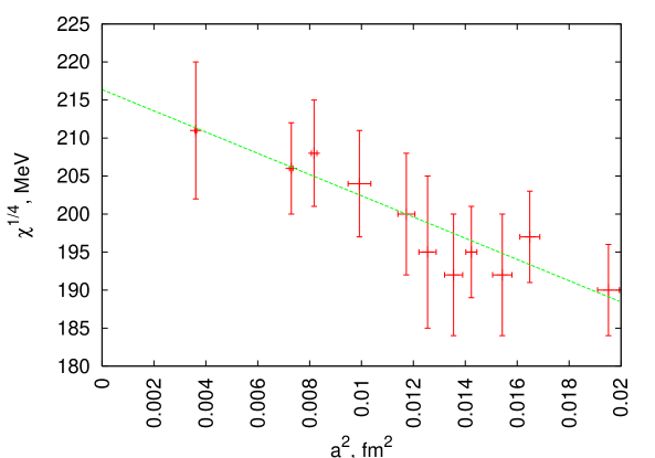
Figure 6: Scaling of the ${\mathrm{HP}^{1}}$-based topological susceptibility with lattice spacing; line is the best fit to Eq. (28).

As far as the lattice spacing dependence of the susceptibility is concerned, it is not a priori evident that $\chi(a)$ is not plagued by power divergences contrary to the case of overlap-based definition. Unfortunately, we’re still lacking the theoretical arguments which could highlight the issue and should rely, in fact, only on the results of the numerical simulations. Note however that at least non-universal $O(a^{2})$ discretization effects are expected generically. Therefore let us consider the topological susceptibility as a function of squared lattice spacing, Fig. 6. As is clear from the figure the dependence $\chi(a^{2})$ is totally compatible with linear one

$$\chi^{1/4}(a^{2})=\chi^{1/4}~{}+~{}\alpha\cdot a^{2}$$ (28)

and does not show any pathology in the limit of small lattice spacing. Of course, the dependence (28) is not guaranteed to persist in the academical limit $a\to 0$, but our data strongly disfavors this possibility. The conclusion is that the topological susceptibility in the ${\mathrm{HP}^{1}}$ approach is not plagued by power divergences. Moreover, the best fit according to Eq. (28) leads to

$$\chi^{1/4}~{}=~{}216(4)\mathrm{~{}MeV}\,,$$ (29)

which is totally compatible with the conventional value of topological susceptibility in the continuum limit (see, e.g., Ref. Lucini:2001ej and references therein). Note that in Ref. Gubarev:2005jm we got $\chi^{1/4}_{overlap}=225(3)\mathrm{~{}MeV}$ on essentially the same configurations using overlap-based definition of the topological charge. We believe that this difference is completely inessential and should be attributed to the finite width of cumulative $Q_{\mathrm{HP}^{1}}$, $Q_{overlap}$ distribution along the line $Q_{\mathrm{HP}^{1}}=-Q_{overlap}$, which we discussed in previous section.

To summarize, our high statistics computation of the topological susceptibility, which was always considered as a testbed for all topological charge constructions, shows that the ${\mathrm{HP}^{1}}$ method is most likely to be free of any lattice related pathology. In particular, we do see almost perfect scaling of $\chi$ within our approach and it does not reveal any sign of necessity of multiplicative renormalization. This provides us a stringent evidence that ${\mathrm{HP}^{1}}$ topological charge is not sensitive to lattice dislocations. As far as the physical results are concerned, the ${\mathrm{HP}^{1}}$ topological susceptibility being extrapolated to the continuum limit is perfectly consistent with the results of other investigations, most notably with overlap-based approach. Keeping in mind all subtleties and technicalities involved in the construction of $Q_{overlap}$ we could dare to claim that the ${\mathrm{HP}^{1}}$ $\sigma$-model embedding method is comparable with overlap based definition and is, in fact, much more advantageous computationally. Moreover, it is not only the tool to investigate the topological aspects of equilibrium vacuum gauge fields. As we show below it naturally allows to study the role of topology related fluctuations in the non-perturbative dynamics of SU(2) Yang-Mills theory.

V ${\mathrm{HP}^{1}}$ $\sigma$-model Induced Gauge Fields

The essence of ${\mathrm{HP}^{1}}$ $\sigma$-model embedding method is the assignment of quaternionic valued scalar fields $\{|\,q_{x}\,\rangle\}$ to the original SU(2) gauge fields configuration. The crucial question here is the uniqueness of this assignment and, unfortunately, in the case of equilibrium gauge fields it seems to be impossible to investigate this issue analytically. However, the results of Ref. Gubarev:2005rs and the ones presented above suggest that non-uniqueness is most likely to be physically irrelevant. Therefore let us assume that the association of $\{|\,q_{x}\,\rangle\}$ with a particular gauge configuration is indeed unique. It is crucial that the corresponding ${\mathrm{HP}^{1}}$ projection

$$U_{x,\mu}~{}\to~{}U^{{\mathrm{HP}^{1}}}_{x,\mu}\equiv\frac{\langle\,q_{x}\,|\,q_{x+\mu}\,\rangle}{|\langle\,q_{x}\,|\,q_{x+\mu}\,\rangle|}$$ (30)

is gauge covariant since under gauge rotations both $U_{x,\mu}$ and $U^{\mathrm{HP}^{1}}_{x,\mu}$ transform exactly in the same way. In this respect the ${\mathrm{HP}^{1}}$ projection is radically distinct from what is usually called ’projection’ in the literature. The very appearance of Eq. (30) was motivated only by consideration of the gauge fields topology and the word ’projection’ here is just the unfortunate terminology. However, this term is in common use and we adopted it also.

Eq. (30) naturally allows to consider the properties of $\{U^{{\mathrm{HP}^{1}}}\}$ fields viewed as usual SU(2) matrices assigned to lattice links. The purpose of this section is to investigate the dynamics of ${\mathrm{HP}^{1}}$ induced gauge fields from various viewpoints. In section V.1 we consider the simplest observable, the gauge curvature of induced potentials, and investigate its dependence upon the lattice spacing. Then the crucial question of confinement in the projected fields is studied in section V.2. Finally in section V.3 the properties of $\{U^{{\mathrm{HP}^{1}}}\}$ configurations are investigated with chirally symmetric overlap Dirac operator. Since this section is rather lengthy and presents quite remarkable results, we conclude it with brief summary (section V.4).

V.1 Gluon Condensate and Quadratic Corrections

The immediate question about ${\mathrm{HP}^{1}}$ induced gauge fields is the corresponding curvature. On the lattice this amount to the consideration of the trace of the plaquette matrix $1/2\mathop{\rm Tr}U^{\mathrm{HP}^{1}}_{p}$ constructed as usual from $U^{\mathrm{HP}^{1}}_{x,\mu}$ and it turns out that ${\mathrm{HP}^{1}}$ induced curvature is astonishingly small, $\langle 1/2\mathop{\rm Tr}U^{\mathrm{HP}^{1}}_{p}\rangle~{}\gtrsim~{}0.97$, on all configurations we have in our disposal. To illustrate this we note that the typical distribution of $1-1/2\mathop{\rm Tr}U^{\mathrm{HP}^{1}}_{p}$ measured on ${\mathrm{HP}^{1}}$ projected configurations is radically different from that on the original fields and is well described by power law, which should be compared with usual almost exponential tail in $1-1/2\mathop{\rm Tr}U_{p}$ distribution. It is amusing that $1-1/2\mathop{\rm Tr}U^{\mathrm{HP}^{1}}_{p}$ distribution looks similar to the lumps volume distribution reported in Gubarev:2005rs and most probably they are indeed closely related. In fact, it is a clear evidence that the dynamics of ${\mathrm{HP}^{1}}$ projected fields is totally different from that of original ones although it is still completely determined by the original Wilson action.

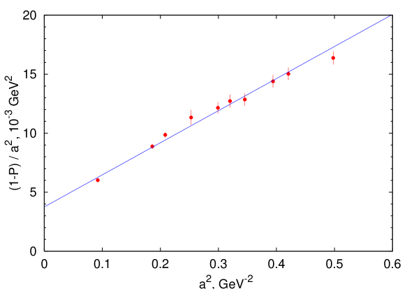
Figure 7: Scaling of averaged plaquette $P=\langle 1/2\mathop{\rm Tr}U^{\mathrm{HP}^{1}}_{p}\rangle$ constructed from ${\mathrm{HP}^{1}}$ projected gauge fields. Line is the best fit according to Eq. (31).

In principle it is an interesting question how the above power law dependence changes with lattice spacing, but we’ll not directly consider it. Instead let us focus on the spacing dependence of averaged plaquette $\langle 1/2\mathop{\rm Tr}U^{\mathrm{HP}^{1}}_{p}\rangle$ for which rather accurate results could easily be obtained. We have measured the ${\mathrm{HP}^{1}}$ induced mean plaquette $\langle 1/2\mathop{\rm Tr}U^{\mathrm{HP}^{1}}_{p}\rangle$ at various spacings quoted in Table 1. The result is presented on Fig. 7 and indeed is quite remarkable. The spacing dependence of $\langle 1/2\mathop{\rm Tr}U^{\mathrm{HP}^{1}}_{p}\rangle$ is totally distinct from what could be expected for unprojected fields and as a matter of fact is astonishingly well described by simple polynomial

$$1~{}-~{}\langle 1/2\mathop{\rm Tr}U^{\mathrm{HP}^{1}}_{p}\rangle~{}=~{}\alpha_{2}\,a^{2}~{}+~{}\alpha_{4}\,a^{4}$$ (31)

throughout the whole range of spacings considered. The justify the assertion (31) we plot on Fig. 7 the dependence of $a^{-2}\cdot(1-\langle 1/2\mathop{\rm Tr}U^{\mathrm{HP}^{1}}_{p}\rangle)$ upon the squared lattice spacing and it is apparent that this dependence is indeed linear. In turn the best fit gives $\chi^{2}/n.d.f.=1.2$ and the optimal values of parameters are

$$\alpha_{2} = [\,61(3)\mathrm{~{}MeV}\,]^{2}\,,$$ (32)

$$\alpha_{4} = 0.0271(10)\mathrm{~{}GeV}^{4}\,.$$

It is quite remarkable that the dependence (31) shown on Fig. 7 by solid line includes only positive powers of lattice spacing. This means, in particular, that $\langle 1/2\mathop{\rm Tr}U^{\mathrm{HP}^{1}}_{p}\rangle$ contains no trace whatsoever of the perturbation theory contribution and is vanishing in the limit $a\to 0$. Thus $1-\langle 1/2\mathop{\rm Tr}U^{\mathrm{HP}^{1}}_{p}\rangle$ could be considered as the definition of non-perturbative contribution present in $\langle\alpha_{s}\,G^{2}/\pi\rangle_{full}$, where we have used the conventional continuum notations and subscript indicates that averaging is done in the full theory including perturbative series. We are in haste to add, however, that at the time being this definition looks completely ad hoc. Indeed, we cannot identify $\langle 1/2\mathop{\rm Tr}U^{\mathrm{HP}^{1}}_{p}\rangle$ as the only non-perturbative part of the $\langle\alpha_{s}\,G^{2}/\pi\rangle_{full}$ until we analyze the content of original gauge fields not surviving ${\mathrm{HP}^{1}}$ projection (30). We will do this in section VI and right now let us agree to treat $\langle 1/2\mathop{\rm Tr}U^{\mathrm{HP}^{1}}_{p}\rangle$ as the genuine non-perturbative quantity. Then it is straightforward to relate the coefficient $\alpha_{4}$, Eq. (31), with gluon condensate $\langle\alpha_{s}\,G^{2}/\pi\rangle$ introduced first in Shifman:1978bx . Indeed, discarding temporally the $O(a^{2})$ term in (31) we have

$$1-\langle 1/2\mathop{\rm Tr}U^{\mathrm{HP}^{1}}_{p}\rangle = \alpha_{4}\,a^{4}(\beta)=$$

$$= a^{4}(\beta)\frac{\pi^{2}}{12\cdot 2}\langle\alpha_{s}\,G^{2}/\pi\rangle\,,$$

thus obtaining the following estimation of the gluon condensate

$$\langle\alpha_{s}\,G^{2}/\pi\rangle~{}=~{}0.066(2)\mathrm{~{}GeV}^{4}\,.$$ (34)

As far as the comparison with existing literature is concerned, let us mention that the gluon condensate being the quantity of prime phenomenological importance is most frequently discussed within the $SU(3)$ pure gauge theory. Here the most recent lattice measurements give $\langle\alpha_{s}\,G^{2}/\pi\rangle_{SU(3)}\approx 0.04\mathrm{~{}GeV^{4}}$ albeit with large uncertainties (see, e.g., Ref. Rakow:2005yn and references therein). This value should be compared with phenomenological one $\langle\alpha_{s}\,G^{2}/\pi\rangle_{SU(3)}\approx 0.012\mathrm{~{}GeV^{4}}$ coming from SVZ sum-rules Shifman:1978bx . We see that even in the most phenomenologically relevant case of $SU(3)$ gauge group the estimations of the gluon condensate vary widely and are, in fact, fairly compatible with (34). If we turn now to the case of $SU(2)$ gauge group, the results which we were able to find in the literature are again in accordance with our estimation (34) and vary from $\langle\alpha_{s}\,G^{2}/\pi\rangle\approx 0.02\mathrm{~{}GeV^{4}}$, Baig:1985pu , to $\langle\alpha_{s}\,G^{2}/\pi\rangle\approx 0.15\mathrm{~{}GeV^{4}}$, DiGiacomo:1981wt (for review see, e.g., Refs. gluon and references therein). Therefore, we are confident that the value of the gluon condensate coming from ${\mathrm{HP}^{1}}$ $\sigma$-model embedding method agrees rather nicely with what is known in both SU(2) and SU(3) cases. Moreover, in view of the well known tremendous uncertainties of usual approaches we conclude that Eq. (34) provides the most accurate estimation of the gluon condensate in $SU(2)$ gauge theory available so far. Note that the systematic errors involved in (34) are coming only from ${\mathrm{HP}^{1}}$ projection (30). However, as we argue in section VI, the systematic uncertainties are most likely to be vanishing thus justifying the estimate (34).

Turn now to the quadratic correction term present in (31). Generically it corresponds to the dimension 2 condensate $\langle A^{2}_{min}\rangle$ which was introduced, in fact, long ago A2-old and became the subject of active development recently Burgio:1997hc ; A2 (see, e.g., Refs. A2-review and references therein). Note however that the theoretical status of quadratic corrections in general and, in particular, the status $O(a^{2})$ correction to the gluon condensate is uncertain at present. Indeed, the quadratic correction to $\langle\alpha_{s}\,G^{2}/\pi\rangle$ was clearly seen in Ref. Burgio:1997hc , however, the corresponding coefficient decreases with increasing number of subtracted perturbative loops A2-plaq and it is by no means evident whether $O(a^{2})$ term has the non-perturbative origin or comes from the higher orders of perturbation theory (see Refs. viz ; viz2 for clear and concise discussion). Generically our data (31) seem to disfavor the perturbative origin of the quadratic term (see also section VI). However, as was argued in Introduction we are not in the position to interpret theoretically this problem and would like to postpone the corresponding analyzes future .

As far as the actual numbers are concerned, it is remarkable that the value of $\alpha_{2}$ coefficient, Eq. (32), is unexpectedly small compared to the natural scale $\Lambda^{2}_{QCD}$, but nevertheless almost fits into the established bounds quoted in Ref. Rakow:2005yn . Note that although the data for $SU(3)$ gauge group was presented in Rakow:2005yn , it seems for us that the parametric smallness of the quadratic correction term is quite generic and should also be valid in $SU(2)$ case. Therefore, we are confident that the estimate (32) is not in contradiction with the most recent literature.

To summarize, the measurements of the curvature of ${\mathrm{HP}^{1}}$ projected gauge fields performed in a wide range of lattice spacings reveal that these potentials are extremely weak compared to that of the original Yang-Mills theory. Moreover, the lattice spacing dependence of averaged ${\mathrm{HP}^{1}}$ plaquette is astonishingly well described by simple power law, Eq. (31), with only $O(a^{4})$ and $O(a^{2})$ terms present and with no sign whatsoever of the perturbation theory contribution. We argued that these terms are to interpreted as the non-perturbative gluon condensate and unusual quadratic power correction to $\langle\alpha_{s}\,G^{2}/\pi\rangle$. The factual absence of perturbative tail in $\langle 1/2\mathop{\rm Tr}U^{\mathrm{HP}^{1}}_{p}\rangle$ allows us to obtain numerically precise estimation of the gluon condensate, which agrees nicely with the existing literature. On the other hand, the measured magnitude of the quadratic term allows to investigate the issue of unusual power corrections in Yang-Mills theory on qualitatively new level. As far as the systematic bias introduced by ${\mathrm{HP}^{1}}$ projection (30) is concerned, we postpone its discussion until section VI and only note here that it is likely to be inessential.

V.2 Confinement in Induced Gauge Fields

In this section we consider the crucial question of confinement in ${\mathrm{HP}^{1}}$ projected gauge fields. In section V.2.1 we discuss the Wilson loops confinement criterium and the scaling properties of ${\mathrm{HP}^{1}}$ projected string tension $\sigma^{\mathrm{HP}^{1}}$. Then we try to identify the objects which seem to be directly related to the non-vanishing $\sigma^{\mathrm{HP}^{1}}$. Finally, in section V.2.3 the Polyakov lines correlation function is considered.

V.2.1 String Tension from Wilson loops

In order to investigate the confinement properties of ${\mathrm{HP}^{1}}$ projected gauge fields (30) we have measured the planar $T\times R$ Wilson loops using various data sets listed in Table 1. As might be expected the weakness of projected fields allows to obtain numerically rather accurate results even without the conventional spatial smearing Albanese:1987ds and hypercubic blocking Hasenfratz:2001hp of temporal links. Indeed, we have checked that the utilization of both these techniques does not change our results in any essential way. However, both these tricks are in fact mandatory to extract the string tension of the original gauge fields to be compared to that on $\{U^{\mathrm{HP}^{1}}\}$ configurations. In order to make the algorithms, applied to the original and ${\mathrm{HP}^{1}}$ projected fields, coherent the smearing and hypercubic blocking was done in both cases. From $\langle W(T,R)\rangle$ the heavy quark potential $V^{\mathrm{HP}^{1}}(R)$ was extracted in standard way (see, e.g. Ref. Bali:1994de for details). In order to obtain the ${\mathrm{HP}^{1}}$ projected string tension $\sigma^{\mathrm{HP}^{1}}$ the potential was fitted to

$$V^{\mathrm{HP}^{1}}(R)~{}=~{}const~{}+~{}\frac{\alpha}{R}~{}+~{}\sigma^{\mathrm{HP}^{1}}\cdot R\,.$$ (35)

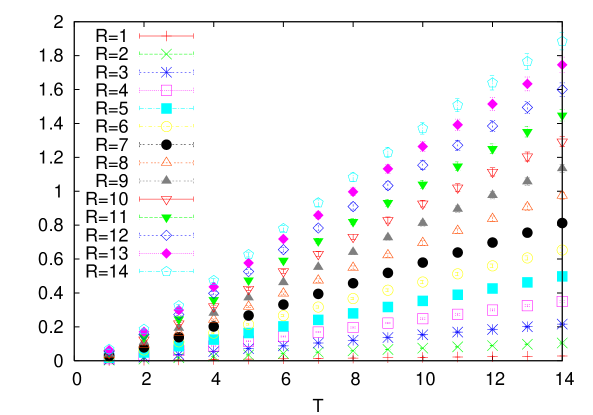
Figure 8: $-\ln\langle W(T,R)\rangle$ as a function of $T$ at various $R$ measured at $\beta=2.600$ on $28^{4}$ lattice.

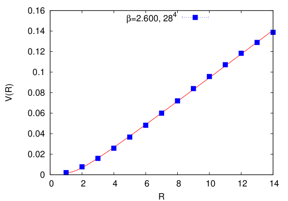
Figure 9: Heavy quark potential $V^{\mathrm{HP}^{1}}(R)$ extracted from Wilson loops measured at $\beta=2.600$ on $28^{4}$ lattice. Solid curve is the fit to Eq. (35).

To convince the reader that despite of the $U^{\mathrm{HP}^{1}}$ fields weakness the potential $V^{\mathrm{HP}^{1}}(R)$ is indeed linearly rising we show on Fig. 8 the behavior of $-\ln\langle W(T,R)\rangle$ as a function of $T$ at various $R$ measured at $\beta=2.600$ on $28^{4}$ lattice. The corresponding potential $V^{\mathrm{HP}^{1}}(R)$ is depicted on Fig. 9. Note that the errors bars here are smaller than the size of symbols. It is apparent that the potential has positive second derivative for $R<4$ which probably indicates the reflection positivity violation. However, we don’t think that this is a real problem. Indeed, the ${\mathrm{HP}^{1}}$ projected gauge fields do not contain the perturbative contribution (see above) and already for this reason are not obliged to fulfill the usual requirements of reflection positivity. Additional argument comes from the intrinsic non-locality of ${\mathrm{HP}^{1}}$ projection. We could only hope to recover the refection positivity in the large distance limit and it is pleasant to note that indeed the potential does not look pathological for $R>3$ ($R\gtrsim 0.2\mathrm{~{}fm}$ in physical units).

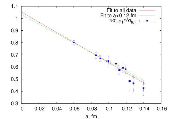
Figure 10: Scaling of ${\mathrm{HP}^{1}}$ projected string tension $\sigma^{\mathrm{HP}^{1}}$ compared to that of full $SU(2)$ string tension $\sigma^{SU(2)}$. Lines are the best fits according to Eq. (36) in the whole range of available spacings and in the region $a<0.12\mathrm{~{}fm}$.

As a matter of fact these plots are typical for all our data sets. The only difference is that at smaller $\beta$-values we don’t see any sign of the reflection positivity violation at small $R$, the potential is everywhere linear within the errors bars. However, the projected string tension depends non-trivially on the lattice spacing. In order to investigate $\sigma^{\mathrm{HP}^{1}}$ scaling properties we calculated the full $SU(2)$ string tension $\sigma^{SU(2)}$ on our configurations and considered the ratio of $\sqrt{\sigma^{\mathrm{HP}^{1}}}$ and $\sqrt{\sigma^{SU(2)}}$. This trick allows us not only to cross-check the physical scale of our fixed volume configurations, but also to avoid the finite volume systematic uncertainties. The resulting plot of the ratio $[\sigma^{\mathrm{HP}^{1}}/\sigma^{SU(2)}]^{1/2}$ with rather pessimistic error estimates as a function of lattice spacing is presented on Fig. 10. It is clear that the scaling of string tensions ratio is fairly compatible with linear $a$-dependence

$$\sqrt{\sigma^{\mathrm{HP}^{1}}}/\sqrt{\sigma^{SU(2)}}~{}=~{}c_{0}~{}+~{}c_{1}\cdot a\,.$$ (36)

Indeed, on general grounds we could exclude the possibility of negative powers of $a$ in (36) while our data is practically insensitive to the inclusion of $O(a^{2})$ terms. Apparently three points corresponding to the largest spacings systematically deviate from (36) which can be attributed the closeness of the crossover transition. Therefore we could try to fit the data to Eq. (36) either in the region $a<0.12\mathrm{~{}fm}$ or in the whole range of available spacings. It turns out that $c_{0}$ value is practically independent upon the concrete choice of the fitting range being $1.03(2)$ and $1.05(2)$ in both cases correspondingly. Therefore the value of the string tensions ratio in the continuum limit is

$$\sqrt{\frac{\sigma^{\mathrm{HP}^{1}}}{\sigma^{SU(2)}}}~{}=~{}1.04(3)\,.$$ (37)

Note that this result is indeed remarkable. Taken at face value it indicates that in the continuum limit the full $SU(2)$ string tension arises solely due to the rather weak ${\mathrm{HP}^{1}}$ projected fields. Simultaneously this is the first indication that what had been cut away from the original fields by ${\mathrm{HP}^{1}}$ projection corresponds likely to pure perturbation theory. On the other hand, Eq. (37) should not come completely unexpected. Indeed, the non-vanishing value of the dimension 2 condensate in ${\mathrm{HP}^{1}}$ projected fields (see section V.1) is a hint that the projected theory might be confining viz ; viz2 ; A2-confine . However, we will not dwell on this issue any longer but consider the anatomy of ${\mathrm{HP}^{1}}$ string tension instead.

V.2.2 String Tension and Topological Fluctuations

One of the central point of Ref. Gubarev:2005rs was rediscovery of the lumpy structure Gattringer ; DeGrand ; Hip ; Horvath of the topological charge density bulk distribution in ${\mathrm{HP}^{1}}$ $\sigma$-model approach. As was stressed in that paper, the term ’lumps’ is in fact uncertain until one introduces a particular cutoff $\Lambda_{q}$ on the magnitude of the local topological charge density. Indeed, the most straightforward argument here is that in the numerical simulations the topological density is always known with finite accuracy and therefore a particular cutoff applies inevitably. Moreover, the introduction of finite $\Lambda_{q}$ is inherent to practically all studies of the gauge fields topology. For instance, the overlap-based topological density, which is given by the sum of Dirac eigenmodes $\psi_{\lambda}$ contributions, is usually either restricted to lowest modes, $\lambda<\Lambda$, or is considered for all modes available on the lattice, $\lambda\lesssim 1/a$. In both cases it is apparent that a particular cut on the topological density is introduced although it might not be simply expressible in terms of $\Lambda$ or $1/a$. Another example of this kind is provided by the investigations of local chirality of Dirac eigenmodes Cundy:2002hv ; Gattringer ; DeGrand ; Hip ; Horvath . Here the local chirality is considered only in points at which the eigenmode is reasonably large.

Then the crucial question is the dependence of physical observables upon $\Lambda_{q}$. The point of view accepted in Ref. Gubarev:2005rs is that this dependence must be trivial since $\Lambda_{q}$ is technical rather than physical parameter. This requirement fixes, in fact, the physically meaningful values of $\Lambda_{q}$ (’physical window’ in the terminology of Ref. Gubarev:2005rs ) which appears to be rather narrow and is around $[300-350\mathrm{~{}MeV}]^{4}$. The attempt to consider the limit $\Lambda_{q}\to 0$ results in rather peculiar structure of topological excitations which is reminiscent to one discovered in Horvath-structures with overlap-based definition of the topological density. Namely, the density of lumps seems to be divergent with $\Lambda_{q}\to 0$ due to the abundance of the lumps consisting of only one lattice site. Simultaneously lumps of larger volumes are accumulating in a few (typically two) percolating lumps with linear extent equal to the size of the lattice. However, both the small lumps distribution and the volume occupied by percolating lumps are strongly $\Lambda_{q}$-dependent and for that reason the small values of the cutoff were excluded in Ref. Gubarev:2005rs from the $\Lambda_{q}$ physical window. It is important that the topological susceptibility remains lumps-saturated even beyond the above percolation transition and essentially this was the justification for the existence of $\Lambda_{q}$ physical window.

It is natural then to ask the same question about the ${\mathrm{HP}^{1}}$ string tension, namely, to consider $\Lambda_{q}$ dependence of $\sigma^{\mathrm{HP}^{1}}$, Eq. (35). Evidently we should confront the $\Lambda_{q}$ physical window found in Gubarev:2005rs with the requirement of $\Lambda_{q}$ independence of $\sigma^{\mathrm{HP}^{1}}$. The first problem to be addressed here is how the string tension could at all be dependent upon the cutoff on the topological density. For the topological susceptibility the solution is trivial, it suffice to consider the small values of the topological density $|q(x)|<\Lambda_{q}$ as being zero exactly. Now we have to formulate the same principle at the level on ${\mathrm{HP}^{1}}$ projected gauge fields maintaining the gauge covariance. The straightforward way to achieve this is provided by Eq. (5). Indeed, every ${\mathrm{HP}^{1}}$ induced link is representable as

$$U^{\mathrm{HP}^{1}}_{x,\mu} = \frac{\langle\,q_{x}\,|\,q_{x+\mu}\,\rangle}{|\langle\,q_{x}\,|\,q_{x+\mu}\,\rangle|}=$$

$$= \bar{g}_{x}\frac{[1;\bar{\omega}_{x}]\,[1;\omega_{x+\mu}]^{T}}{|1+\bar{\omega}_{x}\omega_{x+\mu}|}g_{x+\mu}\equiv\bar{g}_{x}\,h_{x,\mu}\,g_{x+\mu}\,,$$

where $h_{x,\mu}\in SU(2)$ is, in fact, gauge invariant quantity. If the topological density in the vicinity of point $x$ is small, $|q(x)|<\Lambda_{q}$, it is sufficient to equate the inhomogeneous coordinates $\omega_{x}$, $\omega_{x+\mu}$ to each other thus replacing

$$h_{x,\mu}~{}\to~{}1\,,\qquad U^{\mathrm{HP}^{1}}_{x,\mu}~{}\to~{}\bar{g}_{x}\,g_{x+\mu}\,.$$ (39)

This receipt is indeed natural since it maintains gauge covariance and nullifies the contribution of the link $U^{\mathrm{HP}^{1}}_{x,\mu}$ to any Wilson loop. Note however that we are not allowed to change the links and topological density at other points. This means that Eq. (39) should be understood on the level of links only, it is not allowed to actually change neither $|\,q_{x}\,\rangle$ nor $|\,q_{x+\mu}\,\rangle$. Our implementation of this approach is as follows: the $U^{\mathrm{HP}^{1}}_{x,\mu}$ link matrix is transformed according (39) if the magnitude of the topological density in 8 neighboring hypercubes containing the link $\{x,\mu\}$ is smaller than $\Lambda_{q}$.

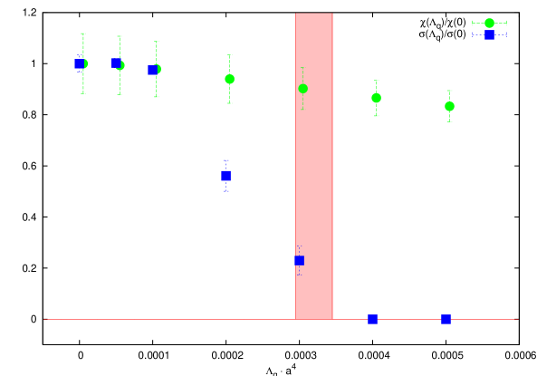
Figure 11: $\Lambda_{q}$ dependence of the ${\mathrm{HP}^{1}}$ string tension (squares) and of the topological susceptibility (circles) both normalized to their respective values at $\Lambda_{q}=0$ ($\beta=2.475$, $16^{4}$). Shaded box stands for the approximate location of the lumps percolation transition (see text).

Unfortunately, the only set of configurations on which we could analyze $\Lambda_{q}$ dependence of $\sigma^{\mathrm{HP}^{1}}$ is the one corresponding to $\beta=2.475$ on $16^{4}$ lattice, thus no scaling checks are possible at the time being. The $\Lambda_{q}$ dependence of the ratios $\sqrt{\sigma^{\mathrm{HP}^{1}}(\Lambda_{q})/\sigma^{\mathrm{HP}^{1}}(0)}$ and $\sqrt{\chi(\Lambda_{q})/\chi(0)}$, where $\sigma^{\mathrm{HP}^{1}}(0)$ and $\chi(0)$ are the ${\mathrm{HP}^{1}}$ string tension and topological susceptibility with no cutoff imposed, is presented on Fig. 11. It is remarkable that the sensitivity of these quantities to the $\Lambda_{q}$ cutoff are radically distinct. The susceptibility decreases only slightly with rising $\Lambda_{q}$ and is changed by $\approx 20\%$ in the whole range of cutoff considered. Contrary to that the ${\mathrm{HP}^{1}}$ string tension drops down to zero at $\Lambda_{q}\cdot a^{4}\approx 3\cdot 10^{-4}$ and remains vanishing for all higher values of the cutoff. Moreover, we cannot exclude the possibility of the phase transition in the infinite volume limit. It is crucial that the string tension vanishes just below the $\Lambda_{q}$ physical window $\Lambda_{q}\cdot a^{4}\in(4\div 8)\cdot 10^{-4}$ discussed in Ref. Gubarev:2005rs . In turn this is not surprising since the ${\mathrm{HP}^{1}}$ string tension was not considered in that paper.

In fact, it is not difficult to identify what happens physically around the point $\Lambda_{q}\cdot a^{4}\approx 3\cdot 10^{-4}$. Indeed, exactly around this value of $\Lambda_{q}$ the percolating lumps cease to exist, the gap separating percolating lumps from the remaining spectrum in the lumps volume distribution disappears. To illustrate this point we indicated the approximate location of the lumps percolation transition by shaded box on Fig. 11. Unfortunately, at present we are not able formulate this qualitative picture more rigorously, mainly because of the limited data we have right now. Nevertheless, we do believe that the disappearance of ${\mathrm{HP}^{1}}$ string tension could be formulated equivalently in the language of lumps percolation transition. The corresponding strong correlation is evident already on our limited data sets and it is probably the question of relatively short time to make this conjecture numerically convincing future .

To summarize, the investigation of ${\mathrm{HP}^{1}}$ string tension dependence on the cutoff imposed on the topological charge density reveals that the string tension is most likely due to the prolongated (extending through all the lattice) regions of sign-coherent topological charge first discovered in Horvath-structures and discussed within ${\mathrm{HP}^{1}}$ approach in Gubarev:2005rs . Therefore the string tension in ${\mathrm{HP}^{1}}$ projected configurations, which accounts for the full $SU(2)$ string tension in the continuum limit, is most sensitive not to the magnitude of the topological density fluctuations, but rather to the long range correlations between them. Contrary to that the topological susceptibility is almost blind to such correlations and, in fact, is saturated by almost random lumps in the topological density bulk distribution.

V.2.3 Polyakov lines correlation function

Let us discuss another conventional confinement indicating observable, namely, the Polyakov line and the corresponding correlation function. The basic observation here is that the Polyakov line ceases to be an order parameter once the gauge potentials (or link matrices in lattice settings) are written as

$$A_{\mu}~{}=~{}\langle\,q\,|\partial_{\mu}|\,q\,\rangle\,,\qquad U_{x,\mu}~{}=~{}\frac{\langle\,q_{x}\,|\,q_{x+\mu}\,\rangle}{|\langle\,q_{x}\,|\,q_{x+\mu}\,\rangle|}\,.$$ (40)

The intrinsic reason for this is that the relevant global center symmetry cannot be formulated in terms of $|\,q_{x}\,\rangle$ fields. Hence the expectation value $\langle P\rangle$ of the Polyakov line is not obliged to vanish in confinement phase once the representation (40) is adopted. Physically this is because it is always possible to form the gauge invariant composite state $|\,q_{x}\,\rangle\psi_{x}$ from $|\,q\,\rangle$ field and quark operator $\psi$. More explicitly, consider for instance the derivation presented Ref. McLerran:1981pb . The equation which is crucial here is the static time-evolution equation

$$(\partial_{t}~{}+~{}A_{0})\,\psi(t,\vec{x})~{}=~{}0\,,$$ (41)

which eventually produces the Polyakov line gauge transporter to be averaged in the thermal ensemble (note that our gauge potentials are anti-hermitian, hence there is no imaginary unit in (41)). Within the representation (40) this equation is equivalent to (we omit the inessential $\vec{x}$ dependence here)

$$\langle\,q_{t}\,|\,\partial_{t}[\,|\,q_{t}\,\rangle\,\psi_{t}\,]~{}=~{}0\,,$$ (42)

which could be solved as

$$\psi_{t}=\langle\,q_{t}\,|\,\int\limits_{0}^{t}[\,|\,q^{\perp}\,\rangle\cdot f\,]~{}+~{}\langle\,q_{t}\,|\,q_{0}\,\rangle\cdot\psi_{0}\,,$$ (43)

where the state $|\,q^{\perp}\,\rangle$ is orthogonal to $|\,q\,\rangle$, $\langle\,q\,|\,q^{\perp}\,\rangle=0$, and is determined, in fact, uniquely, $f$ is arbitrary function and the second term on the r.h.s. is determined from boundary condition at $t=0$. Evidently, for single quark free energy $F_{q}$, considered in the canonical formalism, only the last term does matter (see Ref. McLerran:1981pb for details) and we obtain

$$e^{-F_{q}/T} = \mathop{\rm Tr}[\,e^{-H/T}\,\psi_{1/T}\,\psi^{\dagger}_{0}\,]=$$

$$= \mathop{\rm Tr}[\,e^{-H/T}\,\langle\,q_{1/T}\,|\,q_{0}\,\rangle\,]=1\,,$$

where $H$ is the Hamiltonian, $T$ is the temperature and we assumed that the periodic boundary condition in imaginary time are imposed on the $|\,q\,\rangle$ fields. The result is in agreement with what was noted above: the color charge of both $\psi_{1/T}$ and $\psi_{0}$ gets screened by the quanta of $|\,q\,\rangle$ fields. Note that Eq. (V.2.3) is not dynamical, it is valid irrespectively at both low and high temperatures. Moreover, it confirms that the Polyakov line expectation value $\langle P\rangle$ measured on ${\mathrm{HP}^{1}}$ projected fields is not related to the free energy of static color source and generically is not vanishing at low temperatures

$$\langle P\rangle~{}\neq~{}0\,.$$ (45)

In fact, Eq. (45) is strictly confirmed by our measurements. Depending on the lattice size and spacing $\langle P\rangle$ varies from $\approx 0.42$ to $\approx 0.67$ revealing non-trivial dependence on both $V$ and $a$. However, we did not investigated this dependence due to the uncertainty of its physical implications. On the other hand, the physical meaning of the Polyakov lines connected correlation function is not changing

$$\langle P_{0}\,P_{x}\rangle-\langle P\rangle^{2}~{}\sim~{}\exp\{\,-\frac{1}{T}\,V^{\mathrm{HP}^{1}}(|x|)\,\}\,.$$ (46)

Due to the weakness of ${\mathrm{HP}^{1}}$ projected fields the behavior (46) is firmly confirmed even on the largest lattices we have. It turns out that the potential $V^{\mathrm{HP}^{1}}(R)$ extracted from (46) is in agreement with what we have discussed in section V.2.1 although it has much larger error bars due to the subtraction of disconnected contribution. In particular, it approaches linear asymptotic at large distances, the corresponding string tension being in agreement with that of section V.2.1.

V.3 Chiral Fermions in ${\mathrm{HP}^{1}}$ Projected Gauge Background

It had long been understood that the problem of confinement and chiral symmetry breaking are closely related Gross:1974jv ; fermions-confinement (for recent discussions see, e.g., Refs. fermions-reviews ). In this section we investigate the properties of ${\mathrm{HP}^{1}}$ projected fields (30) as they are seen by fermionic probes provided by the overlap Dirac operator (23). Physically the most important part of the spectrum of (23) is given by low lying eigenmodes

$$D\,\psi_{\lambda}~{}=~{}\lambda\,\psi_{\lambda}\,,$$ (47)

the spectral density $\rho(\lambda)$ of which gives the quenched chiral condensate via Banks-Casher relation banks-casher $\langle\bar{\psi}\psi\rangle~{}=~{}\pi\lim_{\lambda\to 0}\rho(\lambda)$. Another problem of prime importance is the localization properties of low lying modes, which is conventionally formulated in terms of the inverse participation ratio (IPR) $I_{\lambda}$ (see, e.g., Refs. Gubarev:2005jm ; Polikarpov:2005ey ; IPR-defs for definitions). Specifically, we are interested in the scaling of fermionic IPRs with lattice spacing and will not consider dependence upon the total volume (see Refs. Greensite:2005dv for the similar treatment of scalar probe particles). We study both $\rho(\lambda)$ and $I_{\lambda}$ on ${\mathrm{HP}^{1}}$ projected gauge fields obtained from our fixed volume data sets (Table 1) which cover rather wide range of lattice spacings and allow to investigate the scaling of $\rho(\lambda)$ and $I_{\lambda}$ in details. Note that the spacing dependence of IPR for near zero eigenmodes is still the subject of intensive discussions in the literature Gubarev:2005jm ; Polikarpov:2005ey ; IPR-defs . Thus the ${\mathrm{HP}^{1}}$ $\sigma$-model embedding method again provides the unique opportunity to study the issue.

One technical note is now in order. To speed up the calculations we considered only 20 lowest Dirac eigenmodes and excluded the exact zero modes from the analysis since zero modes are known to be physically quite different from the remaining part of the spectrum. This means that we were able to collect the sufficient statistics only for $\lambda\lesssim 400\mathrm{~{}MeV}$ and for this reason all the graphs below are snipped off for higher eigenvalues. However, this does not spoil the significance of our results since exactly the region $\lambda\lesssim 400\mathrm{~{}MeV}$ is most important physically.

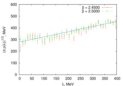
Figure 12: The spectral density of lowest Dirac eigenmodes calculated on fixed volume configurations, Table 1, at different spacings. Line represents linear interpolation towards $\lambda=0$.

Let us consider first the spacing dependence of the spectral density $\rho_{\lambda}$ at small $\lambda$ as is measured on ${\mathrm{HP}^{1}}$ projected gauge fields, Fig. 12. Note that for readability reasons not all available graphs are depicted since the data sets being expressed in physical units look essentially the same at different spacings. It is clear that the points at various $a$ are falling, in fact, on the top of each other thereby confirming that the spectral density of low lying modes is spacing independent. This not only justifies the assertion made earlier that the ${\mathrm{HP}^{1}}$ projection captures correctly the topological aspects of the original gauge fields, but also allows to estimate the quenched chiral condensate

$$\langle\bar{\psi}\psi\rangle~{}=~{}\pi\lim_{\lambda\to 0}\rho(\lambda)~{}=~{}[278(6)\mathrm{~{}MeV}]^{3}\,,$$ (48)

which is in agreement with its value measured on the same original gauge configurations in Ref. Gubarev:2005jm and is fairly compatible with magnitude of $\langle\bar{\psi}\psi\rangle$ known in the literature (see, e.g., Refs. psi-psi and references therein).

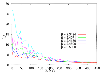
Figure 13: IPRs $I_{\lambda}$ for lowest eigenmodes at various lattice spacings. Note the explicitness of the ’mobility edge’ around $\lambda\approx 200\mathrm{~{}MeV}$.

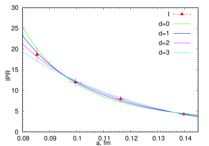
Figure 14: IPR for lowest eigenmodes, Eq. (49), as a function of lattice spacing. The fitting curves (50) are represented by various lines (see text).

As far as the localization properties of lowest eigenmodes are concerned, our results are qualitatively similar to ones reported in Gubarev:2005jm (see also Polikarpov:2005ey ; IPR-defs ). Namely, for $\lambda\lesssim 200\mathrm{~{}MeV}$ the eigenfunctions show notable localization which is apparent from Fig. 13, the corresponding IPRs are ranging from $4\div 8$ at $\lambda\approx 150\mathrm{~{}MeV}$ to $10\div 25$ at smallest non-zero eigenvalues. However, the most important problem is the spacing dependence of $I_{\lambda}$, to study which it is advantageous to consider the IPR averaged over all lowest modes $0<\lambda<\Lambda=50\mathrm{~{}MeV}$

$$I~{}=~{}\frac{1}{N_{\Lambda}}\sum_{\lambda<\Lambda}\,I_{\lambda}\,,$$ (49)

where $N_{\Lambda}$ is the total number of modes in the above interval. This allows to notably improve the statistics, however, we checked that the scaling properties of $I$ are $\Lambda$-independent provided that $\Lambda\lesssim 100\mathrm{~{}MeV}$. The lattice spacing dependence of $I$ allows to investigate quantitatively the dimensionality $d$ of the regions which localize the lowest eigenmodes. As it is customary now (see, e.g., Refs. Gubarev:2005jm ; Polikarpov:2005ey ; IPR-defs for details) we fitted the $I(a)$ dependence to

$$I(a)~{}=~{}b_{0}~{}+~{}b_{1}\cdot a^{d-4}\,,$$ (50)

the best fitting curves for $d=0,1,2,3$ are shown by lines on Fig. 14. Unfortunately, our data does not allow to pinpoint the dimensionality $d$ with high enough accuracy. However, it still favors the two-dimensional structure of the localization regions although we cannot fairly exclude $d=1$ possibility. The relevant $\chi^{2}/n.d.f.$ is equal to $0.33$ for $d=2$ and $0.62$ for $d=1$, while being significantly larger in $d=0$ and $d=3$ cases ($1.26$ and $0.82$ correspondingly). In either case the data is incompatible with naively expected localization on four-dimensional ’balls’ of finite physical extent, the localization volumes are definitely shrinking in the limit $a\to 0$, which is in accord with what is known in the literature Gubarev:2005jm ; Polikarpov:2005ey ; IPR-defs about the low lying fermionic eigenmodes in equilibrium gauge background.

V.4 Summary

Let us briefly summarize the results obtained so far on the dynamics of ${\mathrm{HP}^{1}}$ projected gauge fields. We stress from very beginning that the ${\mathrm{HP}^{1}}$ projection is completely different from what is usually known by the term ’projection’ in the literature. Namely, it maintains the gauge invariance and in view of the investigated irrelevance of Gribov copies problem provides unique gauge invariant variables characterizing the original gauge background. The main conjecture of this section to be justified below is that ${\mathrm{HP}^{1}}$ projected fields represent almost entirely the non-perturbative content of the original gauge fields. We illustrated this point from various perspectives starting from the simplest possible observable, namely, the ${\mathrm{HP}^{1}}$ induced gauge curvature. Remarkably enough, the projected fields appear to be extremely weak, the averaged plaquette $\langle 1/2\mathop{\rm Tr}U^{\mathrm{HP}^{1}}_{p}\rangle$ being distributed with striking power law, which is to be compared with usual exponential distribution. As a consequence, the lattice spacing dependence of $\langle 1/2\mathop{\rm Tr}U^{\mathrm{HP}^{1}}_{p}\rangle$ is totally different from what could be usually expected, we found no sign whatsoever of the perturbation theory in it. As a matter of fact $1-\langle 1/2\mathop{\rm Tr}U^{\mathrm{HP}^{1}}_{p}\rangle$ vanishes in the limit $a\to 0$, the leading spacing corrections being of order $O(a^{4})$ and $O(a^{2})$ only. The corresponding coefficients are to be identified with the gluon condensate and quadratic power correction, both of which we measured with highest accuracy available so far. As far as the gluon condensate is concerned, its value is in a complete agreement with the existing literature. At the same time, the numerically precise value of the quadratic correction given in lattice spacing normalization is reported for the first time and allows to pose the problem of unusual power corrections in Yang-Mills theory on qualitatively new level.

Then we addressed the problem of confinement in the ${\mathrm{HP}^{1}}$ projected gauge fields. Despite of the relative weakness of the ${\mathrm{HP}^{1}}$ induced potentials we showed that the projected theory is still confining. Although at finite lattice spacing the projected string tension is smaller than that on the original fields, it nevertheless reproduces the full $SU(2)$ string tension in the limit $a\to 0$. Moreover, the last statement was found to be quite robust with respect to the technicalities involved. However, it would be plainly wrong to rely on the ${\mathrm{HP}^{1}}$ projection at all distances in particular because the method is practically blind to the perturbation theory. It turns out that the heavy quark potential at small $R\lesssim 0.2\mathrm{~{}fm}$ scales clearly violates the reflection positivity requirements, which, however, is to be expected due to the intrinsic non-locality of ${\mathrm{HP}^{1}}$ $\sigma$-model embedding. We also argued that within our approach the usual confinement sensitive observables like Polyakov line expectation value $\langle P\rangle$ is to be considered with care. In particular, the notion of global center symmetry, which is crucial to ensure $\langle P\rangle=0$ at low temperatures in usual settings, does not exist within the ${\mathrm{HP}^{1}}$ projection method. This clearly rises the question on the relevance of the center symmetry to confinement, however, we postponed the corresponding discussions future and concentrated only on the experimental results instead.

Since the ${\mathrm{HP}^{1}}$ projection is ultimately related to the topology of the gauge fields, it makes possible the investigation of the microscopic origin of the projected string tension. We found that the global (percolating) regions of sign-coherent topological charge Horvath-structures ; Gubarev:2005rs seem to be fundamentally important. Namely, the geometrical explicitness of ${\mathrm{HP}^{1}}$ $\sigma$-model, being superior to any other known topology considerations, allows to scan the gauge fields topology at various scales and to associate rather unambiguously the projected string tension with the existence of the above regions. Note that at present much more data is needed to put the issue on the numerically solid grounds, but for us the correlation is too much evident to be in any doubts.

Finally, in order to present the comprehensive picture of the projected fields dynamics we considered the spectrum of the overlap Dirac operator in the ${\mathrm{HP}^{1}}$ induced background. The observables here are the spectral density of low lying eigenmodes and their localization properties conventionally encoded into inverse participation ratio (IPR). We found that both this quantities are essentially the same as they were on unprojected fields although the actual measurements are much simpler due to the weakness of ${\mathrm{HP}^{1}}$ potentials.

However, the above conclusions rely strongly on the fact that ${\mathrm{HP}^{1}}$ projection leaves aside only the perturbation theory. It is the purpose of the next section to demonstrate that indeed what had been left after the ${\mathrm{HP}^{1}}$ projection likely corresponds to purely perturbative fields.

VI What had been Cut Away by ${\mathrm{HP}^{1}}$ Projection?

The problem to be considered below is the properties of the fields $V_{x,\mu}$ which are the part of original configurations cut away by ${\mathrm{HP}^{1}}$ projection (30). Symbolically $V_{x,\mu}$ could be defined by $V=U/U^{\mathrm{HP}^{1}}$, however, this equation makes no sense as it stands. Indeed, both $U$ and $U^{\mathrm{HP}^{1}}$ transform as usual under the gauge transformations and hence the transformation properties of $V$ are undefined. It is clear that we could make sense of $V$ only in a particular gauge, however, we are not aware of any detailed treatment of this generic problem in the lattice context. The only exception is probably Ref. Bornyakov:2005wp where related issues are discusses. Although the extraction of $V$ variables seems to be similar to the background fields technique, we note that usually the background potentials are taken for granted already in a particular gauge thus invalidating any similarities with the present case.

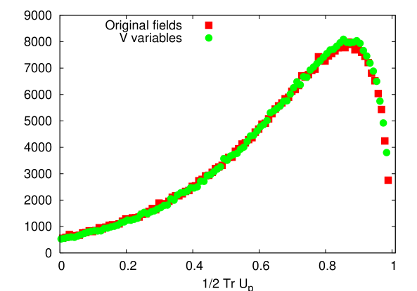
Figure 15: Distribution of trace of the plaquette matrix constructed for a particular configuration ($\beta=2.475$, $16^{4}$) from $U_{x,\mu}$ and $V_{x,\mu}$ fields.

In order to provide the unambiguous meaning to $V_{x,\mu}$ fields we fixed the most convenient and well defined gauge, in which all $|\,q_{x}\,\rangle$ variables are given by the r.h.s. of Eq. (5)

$$|\,q_{x}\,\rangle~{}\to~{}\frac{1}{\sqrt{1+|\omega_{x}|^{2}}}\cdot[\,1\,;\,\omega_{x}\,]^{T}\,.$$ (51)

Then $V_{x,\mu}$ variables are defined by

$$V_{x,\mu}~{}=~{}U_{x,\mu}\cdot\left[U^{\mathrm{HP}^{1}}_{x,\mu}\right]^{\dagger}\,.$$ (52)

Apparently it is important here that $U^{\mathrm{HP}^{1}}_{x,\mu}$ is expressed in terms of factually gauge invariant inhomogeneous coordinates $\omega_{x}$, $\omega_{x+\mu}$. Note that the results to be discussed below are dependent in principle upon the particular gauge chosen, at least we don’t have precise theoretical arguments to exclude this possibility. Since we agreed from very beginning not to go deep into theoretical analysis we leave this problem until the future work future .

In this section we consider the topological aspects of $V$ fields (52), investigate their confining properties and the spectrum of overlap Dirac operator in $V$ fields background. For this purposes we generated $520$ configurations of $V$ fields from the original data sets at $\beta=2.400$ and $\beta=2.475$ on $16^{4}$ lattices. However, let us start again from the simplest observable $1/2\mathop{\rm Tr}V_{p}$ and consider its distribution compared to that of the original fields. The typical graph of this sort, taken on a particular $\beta=2.475$, $16^{4}$ configuration, is presented on Fig. 15. In fact, for all our $V$ configurations the distributions of $1/2\mathop{\rm Tr}V_{p}$ look very similar. Remarkably enough, it is hardly possible to distinguish the points belonging to the original gauge potentials and to $V$ variables, the only difference is seen very close to unity and results in $\lesssim 1\%$ larger value of $\langle 1/2\mathop{\rm Tr}V_{p}\rangle$ on this configuration compared to that of $\langle 1/2\mathop{\rm Tr}U_{p}\rangle$. However, it should not be surprising in view of the above discussed weakness of ${\mathrm{HP}^{1}}$ projected fields. It might be tempting to conclude that the $V$ fields are essentially the same as the original gauge potentials and then the validity of ${\mathrm{HP}^{1}}$ projection would become problematic. However, it is the purpose of this section to show that $V$ fields are completely trivial as far as the non-perturbative aspects are concerned.

VI.1 Triviality of Topological Properties

The technically simplest test of topology is provided by the application of ${\mathrm{HP}^{1}}$ $\sigma$-model embedding method to $V$ configurations. For us it was almost shocking to discover that the $Q_{\mathrm{HP}^{1}}$ topological charge is identically zero for all $V$ configurations we have generated on various lattices. Of course, Eq. (52) expresses our specific intent to cut away the topology related aspects of the original configurations, however, the identically vanishing topological charge is indeed remarkable. Evidently this must be checked by other methods to ensure that $Q\equiv 0$ is not the artifact of ${\mathrm{HP}^{1}}$ approach. We did this cross-check with overlap-based definition and indeed found that $Q_{overlap}$ is equal to $\pm 1$ only on two $V$ configurations out of $520$. Evidently, this disagreement of $Q_{\mathrm{HP}^{1}}$ and $Q_{overlap}$ is completely inessential and should be attributed to what had been discussed in section III. Therefore we are confident that the topological properties of $V$ fields are entirely trivial, the topological charge and susceptibility vanish identically

$$Q\equiv 0\,,\qquad\chi\equiv 0\,.$$ (53)

This is the first indication that what had been left aside by ${\mathrm{HP}^{1}}$ projection is the pure perturbation theory.

VI.2 Loss of Confinement

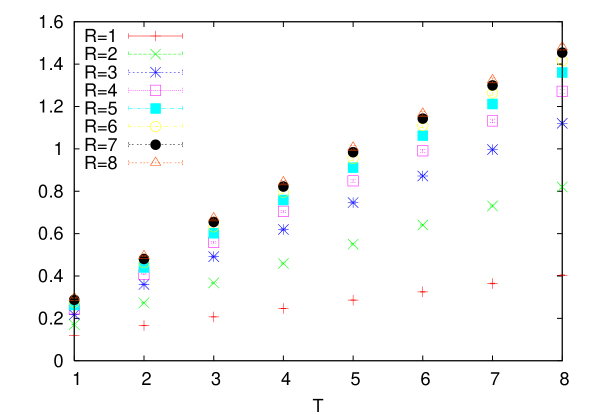
Figure 16: $-\ln\langle W(T,R)\rangle$ as a function of $T$ at various $R$ measured on $V$ configurations generated on $\beta=2.475$, $16^{4}$ lattice.

The next question to be addressed is the possibility to have confinement on $V$ configurations despite of the trivial topology inherent to them. Note that the answer is by no means evident since the relation between topology and confinement is still not proved rigorously. Consider first the Wilson loops confinement criterium. We measured the expectation values of planar $T\times R$ Wilson loops on our $V$ configurations in exactly the same way as was done in section V.2.1. As a matter of fact, on all our $V$ data sets the corresponding heavy quark potential flattens at large distances and the string tension vanishes. In order to convince the reader that the potential is indeed constant at large separations we plotted on Fig. 16 the expectation values $-\ln\langle W(T,R)\rangle$ at various $R$ as a functions of $T$. It is apparent that the slope of the curves remains constant for $R>3$ although it is still rising at smaller distances. The corresponding potential (Fig. 17) was fitted to analytical equation analogous to (35) and turned out to be totally compatible with Coulomb law

$$V(R)~{}=~{}const~{}+~{}\frac{\alpha}{R}\,.$$ (54)

However, we do not presenting the best fitted value of $\alpha$ parameter since on our lattices it would be dictated mostly by $V(R)$ at smallest $R$, which is highly sensitive to the details of smearing and hypercubic blocking used in our calculations (note that essentially for this reason the points $R=1,2$ deviate from (54)).

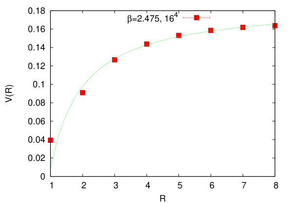
Figure 17: The heavy quark potential extracted from $V$ fields on $\beta=2.475$, $16^{4}$ lattice. The curve is the fit to analytical dependence (54).

As far as the Polyakov line and the corresponding correlation function are concerned, the arguments of section V.2.3 are clearly invalid for $V$ fields and therefore both $\langle P\rangle$ and $\langle P_{0}P_{x}\rangle$ are expected to be the confinement sensitive observables. It turns out that the expectation value $\langle P\rangle$ is strictly positive on all our $V$ data sets being essentially the same at $\beta=2.400$, $\langle P\rangle=0.294(2)$, and at $\beta=2.475$, $\langle P\rangle=0.290(4)$. The strict positivity of Polyakov line distributions apparently rises the question on the relevance of center symmetry, however, due to the possible lack of statistics we’ll not dwell on this issue. The Polyakov lines connected correlation function $\langle P_{0}P_{x}\rangle-\langle P\rangle^{2}$ measured on $V$ configurations also clearly shows deconfining behavior, namely, it falls off only as a power of $|x|$ being strictly linear on log-log plot. Note however that the subtraction of the disconnected part violently spoils the available numerical accuracy and for this reason we do not quote the results of the fits.

To summarize, we found clean evidences that what had been cut away by ${\mathrm{HP}^{1}}$ projection corresponds to deconfining theory, in which the heavy quark potential is totally compatible with Coulomb law. This provides the most stringent illustration that the $V$ fields configurations correspond to pure perturbation theory with no sign whatsoever of neither non-trivial topology nor confinement.

VI.3 Fermionic Probes in $V$ Background

To conclude this section let us consider the properties of low lying eigenmodes of overlap Dirac operator in $V$ fields background. The measurements performed here are essentially the same as was done in section V.3. Note that we considered only $V$ data sets corresponding to $\beta=2.475$ for reasons to become clear shortly.

Figure 18: The spectral density of overlap Dirac operator measured on $V$ fields. Note the complete absence of eigenmodes in $\lambda\lesssim 200\mathrm{~{}MeV}$ interval.

The spectral density of low lying eigenmodes is presented on Fig. 18 and it is apparent that the spectrum is completely empty for $\lambda\lesssim 200\mathrm{~{}MeV}$, no one eigenmode was found in this region on all available $V$ configurations at $\beta=2.475$. Essentially this precludes any considerations of low lying eigenmodes, there are strictly speaking no modes to be discussed here. Thus the spectral density for small $\lambda$ is identically zero leading to vanishing quenched chiral condensate

$$\langle\bar{\psi}\psi\rangle~{}=~{}0\,.$$ (55)

Evidently it makes no sense to discuss the localization properties of low modes in $V$ background, the quantities like $I_{\lambda}$ or $I$, Eq. (49), become undefined. Nevertheless, it is still instructive to qualitatively consider the change in the degree of localization for eigenmodes at $\lambda\gtrsim 200\mathrm{~{}MeV}$ compared to that on the original and ${\mathrm{HP}^{1}}$ projected fields (see section V.3). It turns out that the degree of localization expressed by IPRs $I_{\lambda}$ drop down significantly and for all calculated modes $\lambda\gtrsim 200\mathrm{~{}MeV}$ it is around $1.2$, which essentially means complete delocalization.

VI.4 Summary

In this section we presented rather clean and concise evidences that what had been left aside by ${\mathrm{HP}^{1}}$ projection (30) corresponds to purely perturbation theory. The primary aim of this presentation was to show that the results of section V are not invalidated by the components $V_{x,\mu}$ of the original gauge fields which do not survive ${\mathrm{HP}^{1}}$ projection. We considered this issue from various perspectives and showed that $V$ fields are not confining, the corresponding heavy quark potential is adequately described by usual Coulomb law. Moreover, the topological properties of $V$ configurations are completely trivial, leading, in particular, to the identically vanishing topological susceptibility. This result turns out to be quite robust with respect to different definitions of lattice topological charge. As a consequence the low lying spectrum of overlap Dirac operator in $V$ background has nothing in common with that on the original or ${\mathrm{HP}^{1}}$ projected fields. Strictly speaking, the low lying spectrum does not exist, no one eigenmode was found below $\lambda\lesssim 200\mathrm{~{}MeV}$ despite of rather large number of analyzed configurations. This means that quenched chiral condensate vanishes identically in $V$ background, $\langle\bar{\psi}\psi\rangle=0$.

Therefore, we are confident that the content of the original fields, which is cut away by ${\mathrm{HP}^{1}}$ projection, is completely trivial as far as the non-perturbative aspects are concerned. This provides at least numerically solid grounds for the results obtained in section V.

VII Conclusions

The primary goal of the present publication was the further development of ${\mathrm{HP}^{1}}$ $\sigma$-model embedding approach Gubarev:2005rs aimed to investigate the topology of $SU(2)$ gauge fields. While Ref. Gubarev:2005rs discussed in details the theoretical aspects, the tests of actual numerical implementation were not so much convincing. In this paper we filled this gap and presented the high statistics comparison of ${\mathrm{HP}^{1}}$ based topological charge, $Q_{\mathrm{HP}^{1}}$, with ones obtained via field-theoretical, $Q_{clover}$, and overlap Dirac operator based, $Q_{overlap}$, approaches. As far as the field-theoretical definition is concerned, the corresponding comparison is meaningful only on semiclassical configurations and in this case we essentially found the complete equivalence of $Q_{\mathrm{HP}^{1}}$ and $Q_{clover}$. In the most interesting case of equilibrium vacuum configurations we confronted $Q_{\mathrm{HP}^{1}}$ and $Q_{overlap}$ on rather large number of data sets at different spacings and found that both definitions are strongly correlated and identify essentially the same topology. Unfortunately, it was difficult to compare our results with similar calculations in the literature, however, the correlation between $Q_{\mathrm{HP}^{1}}$ and $Q_{overlap}$ turns out to be quantitatively the same as it was in the case of $Q_{overlap}$ and $Q_{clover}$ definitions. Basing on that we concluded that the ${\mathrm{HP}^{1}}$ $\sigma$-model embedding method is, in fact, computationally superior to any other definitions of the lattice topological charge available so far.

The next immediate problem is to investigate on the numerically confident level the scaling of the topological susceptibility both with lattice spacing and volume. Besides of the methodological importance, this problem is crucial in order to address the physical relevance of the method itself and its sensitivity to lattice artifacts. We performed statistically convincing scaling checks of the topological susceptibility using the ${\mathrm{HP}^{1}}$ embedding approach and found almost perfect scaling with both lattice spacing and volume. The topological susceptibility being extrapolated to the continuum limit turns out to be $\chi^{1/4}=216(4)\mathrm{~{}MeV}$ and is totally compatible with what is known in the literature. The scaling properties of $\chi$ make us confident that the ${\mathrm{HP}^{1}}$ embedding method is insensitive to lattice dislocations, moreover, the topological susceptibility does not require, in fact, neither multiplicative nor additive renormalizations.

As might be anticipated from the results of Ref. Gubarev:2005rs , the ${\mathrm{HP}^{1}}$ embedding approach is not restricted to the topology related measurements. Its essence is to provide a unique (modulo Gribov copies problem which, however, was proved to be inessential) configuration of quaternionic valued scalar fields to any given original gauge background. Then the corresponding ${\mathrm{HP}^{1}}$ projection comes out naturally and we considered in details the properties of ${\mathrm{HP}^{1}}$ projected fields. Note that ${\mathrm{HP}^{1}}$ projection is radically different from what is commonly known by this term, in particular because it maintains the gauge invariance from very beginning. The first striking observation here is that the mean curvature of projected potentials is extremely small, while its spacing dependence shows no sign whatsoever of the perturbation theory. In fact, it only contains the terms which are to be identified with gluon condensate and non-trivial quadratic correction to $\langle\alpha_{s}\,G^{2}/\pi\rangle$. We calculated both this quantities with inaccessible so far accuracy, the result for the gluon condensate being $\langle\alpha_{s}\,G^{2}/\pi\rangle=0.066(2)\mathrm{~{}GeV}^{4}$ which fairly agrees with the existing literature. On the other hand, the numerically precise value of the quadratic correction satisfies the known tight bounds and allows to pose the problem of unusual power corrections in Yang-Mills theory on qualitatively new level.

Then we addressed the crucial problem of confinement in the language of ${\mathrm{HP}^{1}}$ projection. It is remarkable that despite of the weakness of the projected fields the ${\mathrm{HP}^{1}}$ string tension is not only non-zero at finite lattice spacing, it accounts, in fact, for full $SU(2)$ string tension in the continuum limit, $\lim_{a\to 0}[\sigma^{\mathrm{HP}^{1}}/\sigma^{SU(2)}]^{1/2}=1.04(3)$. Moreover, the explicitness of the gauge fields topology in ${\mathrm{HP}^{1}}$ variables allows us to study the microscopic origin of the projected string tension. We argued that $\sigma^{\mathrm{HP}^{1}}\neq 0$ is to be associated with the existence of percolating regions of sign-coherent topological charge, first discovered (with overlap-based approach) in Horvath-structures and then confirmed in ${\mathrm{HP}^{1}}$ method in Gubarev:2005rs . As far as we can see, this is the first explicit demonstration of the confinement-topology interrelation.

We concluded the investigation of ${\mathrm{HP}^{1}}$ projected fields with consideration of low lying spectrum of overlap Dirac operator in the projected background. The spectral density of low eigenmodes turns out to be essentially the same as it was on the original gauge fields and allows us to estimate the value of chiral condensate in the quenched approximation $\langle\bar{\psi}\psi\rangle^{1/3}=278(6)\mathrm{~{}MeV}$, which is fairly compatible with its commonly accepted value. Simultaneously we measured the localization properties of low eigenmodes, which are conventionally expressed in term of the inverse participation ratio (IPR). Knowledge of IPRs at various spacings allows us to conclude that the localization regions are likely to be either two- or three-dimensional.

It was understood from very beginning that the validity of the above results relies strongly on the ability of ${\mathrm{HP}^{1}}$ projection to capture only non-perturbative aspects of the original gauge fields. Therefore it is mandatory to study what had been left aside by ${\mathrm{HP}^{1}}$ projection. We investigated carefully this issue by showing first that the part of the gauge fields not surviving ${\mathrm{HP}^{1}}$ projection could be defined unambiguously. Then it is the matter of straightforward calculation to show that indeed what had been cut away by ${\mathrm{HP}^{1}}$ projection is completely trivial as far as the non-perturbative aspects are concerned. In particular, there is no topology in these fields, the topological charge and susceptibility vanish identically; confinement is definitely lost although the Coulomb part of the potential is clearly seen; and finally the low Dirac spectrum completely disappears, not a single low eigenmode was found on our rather large set of configurations. Thus we concluded that the ${\mathrm{HP}^{1}}$ projection indeed captures only the non-perturbative content of gauge background and what is left aside corresponds to pure perturbation theory.

Finally let us remind our original intent not to discuss the theoretical implications of the above findings. Only experimental numerical results had been reported since otherwise the discussions would definitely lead us far beyond the scope of present publication. The corresponding theoretical treatment is to be published elsewhere future .

References

- (1) H. Neuberger, Phys. Lett. B 417, 141 (1998); Phys. Lett. B 427, 353 (1998).
- (2) M. F. Atiyah and I. M. Singer, Annals Math. 93 (1971) 139.
-
(3)
R. Narayanan and H. Neuberger, Nucl. Phys. B 443, 305 (1995);
P. Hasenfratz, V. Laliena and F. Niedermayer, Phys. Lett. B 427, 125 (1998);
D. H. Adams, Annals Phys. 296, 131 (2002);
R. Narayanan and P. M. Vranas, Nucl. Phys. B 506, 373 (1997). - (4) I. Horvath et al., Phys. Lett. B 612, 21 (2005); Phys. Rev. D 68, 114505 (2003); Nucl. Phys. Proc. Suppl. 129, 677 (2004); A. Alexandru, I. Horvath and J. b. Zhang, Phys. Rev. D 72, 034506 (2005).
- (5) F. V. Gubarev and S. M. Morozov, Phys. Rev. D 72, 76008 (2005).
- (6) M. F. Atiyah, N. J. Hitchin, V. G. Drinfeld and Y. I. Manin, Phys. Lett. A 65, 185 (1978).
- (7) V. G. Drinfeld and Y. I. Manin, Commun. Math. Phys. 63, 177 (1978).
-
(8)
F. Gursey and C. H. Tze, Annals Phys. 128, 29 (1980).
J. Lukierski, CERN-TH-2678;
Y. N. Kafiev, Phys. Lett. B 87 (1979) 219; Phys. Lett. B 96 (1980) 337; Nucl. Phys. B 178, 177 (1981);
M. A. Jafarizadeh, M. Snyder and C. H. Tze, Nucl. Phys. B 176, 221 (1980);
D. Maison, MPI-PAE/PTh 52/79;
J. E. Avron, L. Sadun, J. Segert and B. Simon, Comm. Math. Phys. 124, 595 (1989);
M. T. Johnsson and I. J. R. Aitchison, J. Phys. A 30, 2085 (1997);
E. Demler and S. C. Zhang, Annals Phys. 271, 83 (1999). - (9) B. A. Dubrovin, A. T. Fomenko, S. P. Novikov, “Modern Geometry: Methods and Applications”, “Modern Geometry: Introduction to Homology Theory”, New York: Springer-Verlag (1992).
- (10) F. V. Gubarev, S. M. Morozov, M. I. Polikarpov and V. I. Zakharov, “Low lying eigenmodes localization for chirally symmetric Dirac operator”, hep-lat/0505016, to be published in JETP Letters.
- (11) M. I. Polikarpov, F. V. Gubarev, S. M. Morozov and V. I. Zakharov, ’Localization of low lying eigenmodes for chirally symmetric Dirac operator’, arXiv:hep-lat/0510098.
-
(12)
F. V. Gubarev, L. Stodolsky and V. I. Zakharov, Phys. Rev. Lett. 86, 2220 (2001);
F. V. Gubarev and V. I. Zakharov, Phys. Lett. B 501, 28 (2001);
D. Dudal, H. Verschelde, J. A. Gracey, V. E. R. Lemes, M. S. Sarandy, R. F. Sobreiro and S. P. Sorella, JHEP 0401, 044 (2004);
F. V. Gubarev and S. M. Morozov, Phys. Rev. D 71, 114514 (2005);
D. V. Bykov and A. A. Slavnov, ’“Dimension two vacuum condensates in gauge-invariant theories’, arXiv:hep-th/0505089;
X. d. Li and C. M. Shakin, Phys. Rev. D 71, 074007 (2005);
D. Dudal, R. F. Sobreiro, S. P. Sorella and H. Verschelde, Phys. Rev. D 72, 014016 (2005). -
(13)
V. I. Zakharov, AIP Conf. Proc. 756, 182 (2005);
V. I. Zakharov, Phys. Usp. 47 (2004) 37. -
(14)
F. V. Gubarev, M. I. Polikarpov and V. I. Zakharov, Surveys High Energ. Phys. 15, 89 (2000);
V. I. Zakharov, ’From confining fields back to power corrections’, arXiv:hep-ph/0509114;
V. I. Zakharov, ’Hints on dual variables from the lattice SU(2) gluodynamics’, arXiv:hep-ph/0309301. -
(15)
V. I. Zakharov, ’Confining fields in lattice SU(2)’, arXiv:hep-ph/0312210;
V. I. Zakharov, ’Non-perturbative match of ultraviolet renormalon’, arXiv:hep-ph/0309178. - (16) P.Yu. Boyko, F.V. Gubarev, S.M. Morozov, in preparation.
-
(17)
P. de Forcrand and M. D’Elia, Phys. Rev. Lett. 82, 4582 (1999);
J. Gattnar et al., Nucl.Phys. B716, 105 (2005);
A. V. Kovalenko, M. I. Polikarpov, S. N. Syritsyn and V. I. Zakharov, Phys. Lett. B 613, 52 (2005). - (18) V. G. Bornyakov, M. I. Polikarpov, T. Suzuki and S. N. Syritsyn, AIP Conf. Proc. 756 (2005) 463.
- (19) A. S. Kronfeld, M. L. Laursen, G. Schierholz and U. J. Wiese, Nucl. Phys. B 292, 330 (1987).
- (20) B. Lucini and M. Teper, JHEP 0106, 050 (2001).
-
(21)
J. Fingberg, U. M. Heller and F. Karsch, Nucl. Phys. B 392, 493 (1993);
G. S. Bali, K. Schilling and A. Wachter, Phys. Rev. D 55, 5309 (1997);
G. S. Bali, K. Schilling and C. Schlichter, Phys. Rev. D 51, 5165 (1995). - (22) P. Di Vecchia, K. Fabricius, G. C. Rossi and G. Veneziano, Nucl. Phys. B 192, 392 (1981); Phys. Lett. B 108, 323 (1982).
- (23) N. Cundy, M. Teper and U. Wenger, Phys. Rev. D 66, 094505 (2002).
- (24) M. Garcia Perez, O. Philipsen and I. O. Stamatescu, Nucl. Phys. B 551, 293 (1999).
- (25) S. O. Bilson-Thompson, D. B. Leinweber and A. G. Williams, Annals Phys. 304, 1 (2003).
- (26) P. de Forcrand, M. Garcia Perez and I. O. Stamatescu, Nucl. Phys. B 499, 409 (1997).
- (27) L. Giusti, C. Hoelbling, M. Luscher and H. Wittig, Comput. Phys. Commun. 153, 31 (2003).
-
(28)
T. W. Chiu and S. V. Zenkin, Phys. Rev. D 59, 074501 (1999);
T. W. Chiu, C. W. Wang and S. V. Zenkin, Phys. Lett. B 438, 321 (1998). - (29) S. Capitani, M. Gockeler, R. Horsley, P. E. L. Rakow and G. Schierholz, Phys. Lett. B 468, 150 (1999).
- (30) L. Giusti, M. Luscher, P. Weisz and H. Wittig, JHEP 0311, 023 (2003).
- (31) M. A. Shifman, A. I. Vainshtein and V. I. Zakharov, Nucl. Phys. B 147, 385 (1979); Nucl. Phys. B 147, 448 (1979).
- (32) P. E. L. Rakow, ’Stochastic perturbation theory and the gluon condensate’, arXiv:hep-lat/0510046.
- (33) M. Baig, ’Gluon Condensation Parameter In SU(2) Lattice Gauge Theory And Large N Universality’, UAB-FT-124.
- (34) A. Di Giacomo and G. C. Rossi, Phys. Lett. B 100, 481 (1981).
-
(35)
T. Banks, R. Horsley, H. R. Rubinstein and U. Wolff, Nucl. Phys. B 190, 692 (1981);
S. s. Xue, Phys. Lett. B 191, 147 (1987);
B. Alles, M. Campostrini, A. Feo and H. Panagopoulos, Phys. Lett. B 324, 433 (1994);
A. Di Giacomo,’Non perturbative QCD’, arXiv:hep-lat/9912016;
K. Langfeld, E. M. Ilgenfritz and H. Reinhardt, Nucl. Phys. B 608, 125 (2001). -
(36)
J. Greensite and M. B. Halpern, Nucl. Phys. B 271, 379 (1986);
M. J. Lavelle and M. Schaden, Phys. Lett. B 208, 297 (1988);
M. Lavelle and M. Oleszczuk, Mod. Phys. Lett. A 7 (1992) 3617. - (37) G. Burgio, F. Di Renzo, G. Marchesini and E. Onofri, Phys. Lett. B 422, 219 (1998).
-
(38)
F. Di Renzo and L. Scorzato, JHEP 0110, 038 (2001);
R. Horsley, P. E. L. Rakow and G. Schierholz, Nucl. Phys. Proc. Suppl. 106, 870 (2002). - (39) M. Albanese et al. [APE Collaboration], Phys. Lett. B 192, 163 (1987).
- (40) A. Hasenfratz and F. Knechtli, Phys. Rev. D 64, 034504 (2001) [arXiv:hep-lat/0103029].
- (41) G. S. Bali, K. Schilling and C. Schlichter, Phys. Rev. D 51, 5165 (1995).
-
(42)
K. Ishiguro et al.,
’Towards SU(2) invariant formulation of the monopole confinement mechanism’, arXiv:hep-lat/0509089;
V. I. Shevchenko, ’A remark on the short distance potential in gluodynamics’, arXiv:hep-ph/0301280;
K. I. Kondo, Phys. Lett. B 514, 335 (2001);
H. Verschelde, K. Knecht, K. Van Acoleyen and M. Vanderkelen, Phys. Lett. B 516, 307 (2001);
T. Suzuki, K. Ishiguro, Y. Mori and T. Sekido, Phys. Rev. Lett. 94, 132001 (2005);
M. N. Chernodub et al., Phys. Rev. D 72, 074505 (2005). - (43) C. Gattringer, M. Gockeler, P. E. L. Rakow, S. Schaefer and A. Schafer, Nucl. Phys. B 617, 101 (2001); Nucl. Phys. B 618, 205 (2001).
- (44) T. DeGrand and A. Hasenfratz, Phys. Rev. D 64, 034512 (2001); Phys. Rev. D 65, 014503 (2002).
- (45) I. Hip, T. Lippert, H. Neff, K. Schilling and W. Schroers, Phys. Rev. D 65, 014506 (2002); R. G. Edwards and U. M. Heller, Phys. Rev. D 65, 014505 (2002); T. Blum et al., Phys. Rev. D 65, 014504 (2002).
-
(46)
I. Horvath et al., Phys. Rev. D 66, 034501 (2002);
I. Horvath, N. Isgur, J. McCune and H. B. Thacker, Phys. Rev. D 65, 014502 (2002). - (47) L. D. McLerran and B. Svetitsky, Phys. Rev. D 24, 450 (1981).
- (48) D. J. Gross and A. Neveu, Phys. Rev. D 10, 3235 (1974).
-
(49)
E. Witten, Nucl. Phys. B 149, 285 (1979); Nucl. Phys. B 156, 269 (1979);
A. Casher, Phys. Lett. B 83, 395 (1979). -
(50)
H. G. Dosch and Y. A. Simonov, Phys. Atom. Nucl. 57, 143 (1994) [Yad. Fiz. 57N1, 152 (1994)];
Y. A. Simonov, ’Chiral symmetry breaking and confinement in QCD’, talk given at 31st International Ahrenshoop Symposium on the Theory of Elementary Particles, Buckow, Germany, 2-6 Sep 1997;
K. E. Cahill, ’Chiral symmetry and quark confinement’, arXiv:hep-ph/9812312. - (51) T. Banks, A. Casher, Nucl. Phys. B 169, 103 (1980).
-
(52)
C. Aubin et al. [MILC Collaboration],
’The scaling dimension of low lying Dirac eigenmodes and of the topological charge density’,
arXiv:hep-lat/0410024;
C. Gattringer, M. Gockeler, P. E. L. Rakow, S. Schaefer and A. Schafer, Nucl. Phys. B 617, 101 (2001);
Y. Koma, E. M. Ilgenfritz, K. Koller, G. Schierholz, T. Streuer and V. Weinberg, Proc. Sci. LAT2005, 300 (2005);
C. Bernard et al., ’More evidence of localization in the low-lying Dirac spectrum’, arXiv:hep-lat/0510025;
- (53) J. Greensite, S. Olejnik, M. Polikarpov, S. Syritsyn and V. Zakharov, Phys. Rev. D 71, 114507 (2005); Proc. Sci. LAT2005, 325 (2005), [arXiv:hep-lat/0509070].
-
(54)
S. J. Hands and M. Teper, Nucl. Phys. B 347, 819 (1990);
E. Follana, A. Hart, C. T. H. Davies and Q. Mason [HPQCD Collaboration], Phys. Rev. D 72, 054501 (2005);
L. Giusti, F. Rapuano, M. Talevi and A. Vladikas, Nucl. Phys. B 538, 249 (1999).