Physics prospects of UV-filtered overlap quarks

Abstract

Some key features of the overlap operator with a UV-filtered Wilson kernel are discussed. The first part concerns spectral properties of the underlying shifted hermitean Wilson operator and the relation to the observed speedup of the overlap construction. Next, the localization of the filtered overlap and its axial-vector renormalization constant are discussed. Finally, results of an exploratory scaling study for $m_{ud},m_{s}$ and $f_{\pi},f_{K}$ are presented.

1 INTRODUCTION

On the conceptual level the quest for exact chiral symmetry at finite lattice spacing has been completed. The closely related domain-wall (in the limit $L_{5}\!\to\!\infty$) [1] and overlap [2] approach and also the parametrized fixed point action (in the limit of perfect parametrization) [3] yield lattice fermions which satisfy the Ginsparg-Wilson relation with on-shell chiral symmetry [4]

$$\gamma_{5}D+D\hat{\gamma}_{5}=0\;,\qquad\hat{\gamma}_{5}=\gamma_{5}(1-{1\over\rho}D)\;.$$ (1)

The salient features of such fermions include:

• Additive mass renormalization is absent [4].

• There is an index theorem linking $n_{+}-n_{-}$ (where $n_{\pm}$ is the number of zero-modes of the massless Dirac operator $D$ with $\gamma_{5}\!=\!\pm 1$) to the gluonic topological charge $q$ on fine enough lattices [5].

• The Nielsen-Ninomiya theorem is evaded [6].

• Using “chirally rotated” quark fields to construct e.g. pseudoscalar densities and axialvector currents (see below) the theory has only $O(a^{2})$ cut-off effects [7].

On a practical level the question how one may implement any such scheme at bearable cost in terms of CPU time remains a topic of active research. Considering the massless overlap operator

$$D_{\mathrm{ov}}=\rho\big{[}1+D_{\mathrm{W},-\rho}\big{(}D_{\mathrm{W},-\rho}^{\dagger}D_{\mathrm{W},-\rho})^{-1/2}\big{]}$$ (2)

with $D_{\mathrm{W},-\rho}\!=\!D_{\mathrm{W}}\!-\!\rho$ the shifted Wilson operator ($0\!<\!\rho\!<\!2$) as an example, two avenues are being pursued. One question is what is the numerically most efficient way to implement the $(.)^{-1/2}$ operator prescription in (2). The second strategy is to ask whether a slight modification of the formulation can reduce the computational burden.

2 OVERLAP WITH UV-FILTERING

An obvious idea is to do some “massage” to the Wilson kernel in the overlap prescription, since there is nothing specific to the (plain) $D_{\mathrm{W}}$ in (2); any legal doubler-free fermion action will do fine.

There is a long history of “designer actions” tailored to have a spectrum sufficiently close to the GW circle, such that the inverse squareroot in (2) would minimize the number of forward applications of the kernel on a source vector [8]. These actions typically invoke tunable parameters and the improvement is achieved through additional couplings, i.e. a single row or column of $D$ involves more than the $51$ entries (for $SU(3)$ and chiral repr.) of $D_{\mathrm{W}}$. Hence the challenge is to assess the effect of fewer forward applications versus each application getting more expensive.

In addition, there is quite some experience with filtered actions (including the overlap) [9, 10, 11, 12] where only the covariant derivative is replaced,

$$U_{\mu}(x)\psi(x\!+\!\hat{\mu})\!-\!\psi(x)\to V_{\mu}(x)\psi(x\!+\!\hat{\mu})\!-\!\psi(x)\;,$$ (3)

tantamount to a change by an irrelevant operator. Here, $V_{\mu}(x)$ is defined via an APE [13], HYP [10] or stout-link [14] recipe. The point is that this maintains the sparseness of the Wilson operator and yet a significant speedup can be achieved. The obvious concern is that the filtering might impair the localization properties of the final $D$.

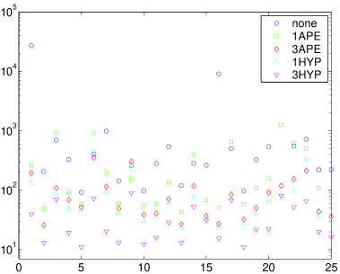
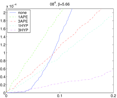
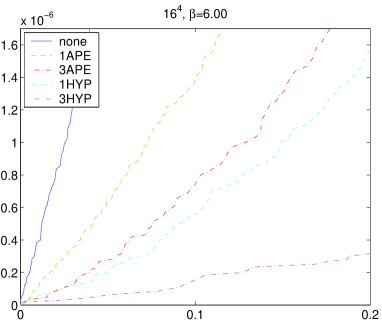
Figure 1: Condition number $1/\epsilon$ of $|H_{\mathrm{W},-\rho}|$ at $\rho\!=\!1$ on 25 quenched $\beta\!=\!6.0$, $16^{4}$ configurations without (left) and with projection of the 14 lowest eigenmodes (right). Modest filtering significantly reduces $1/\epsilon$.

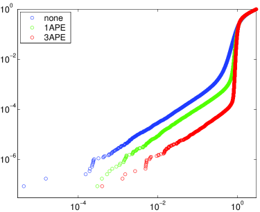
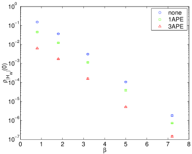
Figure 2: Cumulative eigenvalue distribution of $|H_{\mathrm{W},-\rho}|$ at $\rho\!=\!1$ for $\beta\!=\!5.66$ (left) and $\beta\!=\!6.00$ (right) with 0,1,3 steps of APE or HYP filtering. This reduces the slope and thus $\rho(0)$, but the latter quantity remains non-zero. Evidently, the unfiltered operator at $\beta\!=\!5.66$ is in the wrong universality class.

Figure 3: Cumulative eigenvalue distribution (log-log plot) of $|H_{\mathrm{W},-\rho}|$ in the Schwinger model (${N_{\!f}}\!=\!0$, $16^{2}$, $\beta\!=\!3.2$, $\rho\!=\!1$) with 0,1,3 filtering steps (left) and the pertinent $\rho(0)$ as a function of $\beta$ (right).

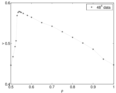
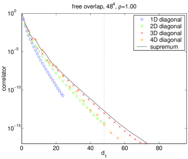
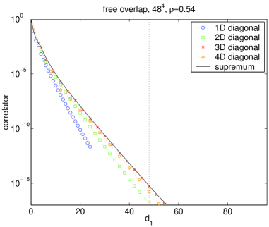
Figure 4: Localization $\nu$ versus $\rho$ at $\beta\!=\!6.0$ without filtering and after 1 step of APE/HYP smoothing (left) and the same relation in the free theory (right); here the optimum $\rho$ is significantly smaller than 1.

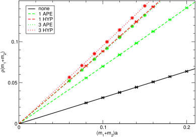
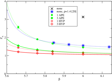
Figure 5: Fall-off pattern (vs. “taxi driver” distance $d_{1}$) of the free overlap operator on-axis (open circles) and for several directions (other symbols) with supremum (full line) at $\rho=1$ (left) and $\rho=0.54$ (right).

Figure 6: AWI mass versus bare mass at $\beta\!=\!6.0$ and $\rho\!=\!1$ for several filtering recipes (left). The quadratic fits are unconstrained and still go through zero, indicating good chiral symmetry. The inverse slope $Z_{A}$ versus $\beta$ (right) shows a much milder dependence with filtering than without, even with $\rho\!=\!1$ kept fixed.

2.1 Spectral properties of $|H_{\mathrm{W},-\rho}|$

We now focus on how the speedup of the overlap construction with UV-filtering can be understood in terms of the spectrum of the underlying hermitean Wilson operator $H_{\mathrm{W},-\rho}\!=\!\gamma_{5}(D_{\mathrm{W}}\!-\!\rho)$. We use the Wilson gauge action, and for technical details we refer to the original publication [15].

The numerical effort to construct the massless operator (2) is in good approximation proportional to the condition number $1/\epsilon$ of $|H_{\mathrm{W},-\rho}|$. Fig. 1 shows $1/\epsilon$ on 25 quenched configurations at $\beta\!=\!6.0$. Evidently, the condition numbers get dramatically reduced through any type of filtering. In practice, overlap calculations use the projection trick, i.e. the subspace pertinent to the lowest few eigenvalues is treated exactly [16]. The interesting news is that even after this trick has been applied, the condition number in the orthogonal complement is improved through filtering (right panel). The data are for $\rho\!=\!1$, with $\rho\!>\!1$ the saving is slightly smaller.

It has been argued that the spectral density of $|H_{\mathrm{W},-\rho}|$ getting too large will eventually make the overlap construction break down on coarse lattices [17]. Fig. 2 shows the cumulative eigenvalue distribution (CED) of $|H_{\mathrm{W},-\rho}|$ with $\rho\!=\!1$ on an extremely coarse ($\beta=5.66$) and a fairly smooth ($\beta\!=\!6.0$) lattice. The slope at the origin is the quantity of interest, $\rho(0)$. The filtering clearly reduces $\rho(0)$, but by no means does it reduce it to zero. A point worth noticing is that the unfiltered CED on the coarse lattice has a rather different shape. At strong coupling the radii of the Wilson spectrum are considerably smaller than 1, and our choice to keep the shift parameter $\rho\!=\!1$ fixed lets us “loose” the fermion. In summary, the overlap construction breaks down on too coarse lattices, but the good news is that $(i)$ one would notice from the CED and ($ii$) the breakdown gets delayed through filtering ($\beta\!=\!5.66$ seems fine if at least 1 filtering step is applied).

Another question is what happens to the spectral density at weak coupling. Fig. 3 shows the CED of $|H_{\mathrm{W},-\rho}|$ in 2D in a log-log representation. With filtering a much higher fraction of the eigenvalues is near $\lambda\!=\!1$, and in this sense the picture is similar to what one would get if one were to use an approximately chiral kernel – in that case the “mobility edge” would be at $\lambda\!=\!1$ and $\rho(0)\!=\!0$. The high statistics study in 2D presented on the right suggests that $\rho(0)$ decays exponentially in $\beta$ and that filtering continues to reduce $\rho(0)$ in the weak coupling regime.

2.2 Localization properties of $D_{\mathrm{ov}}$

It is evident from (2) that $D_{\mathrm{ov}}$ cannot be ultralocal, but the question is whether it is local, i.e. whether the couplings in $D_{\mathrm{ov}}(x,y)$ would decay exponentially in $|x\!-\!y|$ (in some norm). This is important to guarantee that LQCD with $D_{\mathrm{ov}}$ is in the right universality class.

We measure the localization function [18]

$$f(d_{1})=\mathrm{sup}\Big{\{}||(D_{\mathrm{ov}}\eta)(x)||_{2}\;\Big{|}\;||x\!-\!0||_{1}\!=\!d_{1}\Big{\}}$$ (4)

with $\eta$ a normalized source vector at the origin. Here, $d_{1}$ is the distance in the “taxi driver” metric. The localization $\nu$ is the “effective mass” of $f(d_{1})$ for a $d_{1}$ which is sufficiently far from the maximal one ($2L$ in a $L^{4}$ box) to avoid finite volume effects. Fig. 4 shows a scan of $\nu$ as a function of the shift parameter $\rho$ at $\beta\!=\!6.0$. Without filtering the optimized $\rho$ is near $1.4$ [18]. After just 1 APE step the extremum shifts towards $\rho\!\simeq\!1$ and with 1 HYP step it is near $\rho\!\simeq\!0.8$. This finding should not come as a surprise, since in the free theory a value $\nu_{\mathrm{max}}\!\simeq\!0.58$ is realized for $\rho_{\mathrm{opt}}\!\simeq\!0.54$. We consider this a strong rationale for not tuning $\rho$ to an “optimum” value at some standard coupling but for staying with the canonical choice $\rho\!=\!1$. In passing we note that $\rho\!=\!1$ would also minimize the condition number of $|H_{\mathrm{W},-\rho}|$ in the free field limit.

Our choice to use the “taxi driver” distance was motivated by the standards in the literature [18]. Fig. 5 shows $f(d_{1})$ in the free theory for several directions (on-axis and space-diagonals) together with the supremum. One notices that the slope in the 2D-diagonal direction is roughly a factor $\sqrt{2}$ smaller than on-axis, in the 3D-diagonal direction (the one which dominates the supremum) it is about a factor $\sqrt{3}$. In other words, if we had chosen the “beeline” metric $||.||_{2}$, then the maximum localization in the free-field case would have turned out to be roughly $0.58\sqrt{3}\!\simeq\!1$.

2.3 Axialvector renormalization for $D_{\mathrm{ov}}$

In phenomenological studies theoretical uncertainties of lattice-to-continuum renormalization factors often limit the precision of the final answer. In this respect it seems important that such factors would be close to 1 or (at least) show a mild dependence on the gauge coupling.

We determine $Z_{A}$ via the axial Ward identity (AWI). Specifically, we use the “chirally rotated” quark fields [7] to construct the pseudoscalar density and the (naive) axialvector current

$$P(x)\! \!=\! \!\overline{\psi}_{1}(x)\gamma_{5}\big{[}\big{(}1-{a\over 2\rho}D_{\mathrm{ov}}\big{)}\psi_{2}\big{]}(x)$$ (5)

$$A_{\mu}(x)\! \!=\! \!\overline{\psi}_{1}(x)\gamma_{\mu}\gamma_{5}\big{[}\big{(}1-{a\over 2\rho}D_{\mathrm{ov}}\big{)}\psi_{2}\big{]}(x)$$ (6)

where below the fields (flavors) $\psi_{1,2}$ will be taken as solutions to the massive overlap operator

$$D_{\mathrm{ov},m}=\Big{(}1-{am\over 2\rho}\Big{)}D_{\mathrm{ov}}+m$$ (7)

with mass $m_{1,2}$, respectively. The “rotating” operator [7] in (5,6) is still the massless one. With these at hand one forms the ratio

$$\rho(t,m_{1},m_{2})={\sum_{\mathbf{x}}\langle P(\mathbf{x},t)P^{c}(\mathbf{0},0)\rangle\over\sum_{\mathbf{x}}\langle\bar{\nabla}_{\!4}\!A_{4}(\mathbf{x},t)P^{c}(\mathbf{0},0)\rangle}$$ (8)

which yields the sum of the AWI quark masses,

$$\rho(t,m_{1},m_{2})\stackrel{{\scriptstyle t\to\infty}}{{\longrightarrow}}m_{1}^{\mathrm{AWI}}\!+\!m_{2}^{\mathrm{AWI}}+O(a^{2})\;.$$ (9)

Fig. 6 shows the plateau value $\rho(m_{1}\!+\!m_{2})$ for a variety of $(m_{1},m_{2})$ combinations versus the sum $m_{1}\!+\!m_{2}$. Since each $m_{1}\!+\!m_{2}$ is realized in various combinations and we see no spread, we conclude that isospin is a perfect symmetry (in this ratio and within our statistical precision). Using

$$\rho=\mathrm{const}+{1\over Z_{A}}(m_{1}\!+\!m_{2})+\mathrm{const}\,(m_{1}\!+\!m_{2})^{2}$$

as our fit ansatz, we determine the offset at the origin and $Z_{A}$. The former is consistent with zero, and this means that we have indeed good chiral symmetry. How the $Z_{A}$ factors would depend on the gauge coupling is shown on the right. Our data are for $\rho\!=\!1$ and stem from [15, 19]. The data for $\rho\!=\!1.4$ come from [20]. This compilation shows that already a single HYP step at fixed $\rho\!=\!1$ manages to tame the $\beta$-dependence of $Z_{A}$ in a more efficient way than carefully tuning $\rho$ could possibly do. In fact, the $Z_{A}$ values of the filtered overlap are so close to 1 that even a perturbative evaluation at the 1-loop level might work fine (as was done, for a different operator, in [21]).

2.4 Technical summary

Given the discussion in the two previous subsections it is clear that the UV-filtering does not only serve the purpose of speeding up the overlap construction, it really improves the physics properties of the resulting $D_{\mathrm{ov}}$. Let us take the opportunity to highlight some technical points:

• Filtering yields an $O(a^{2})$-redefinition of the overlap (at fixed $\rho,\alpha_{\mathrm{smear}},N_{\mathrm{iter}}$).

• The implementation effort is minimal; just evaluate $D_{\mathrm{ov}}$ on a smeared copy of the original gauge configuration.

• The idea is well-suited for dynamical simulations with HMC [22], provided the stout-link recipe [14] is used.

• The advantages are independent of how the $(.)^{-1/2}$ prescription is implemented and naturally carry over to the domain-wall [1] or Moebius [23] varieties.

Regarding point (a) it should be clear that there is no conflict with the statement in [5, 6] that “the” overlap yields a sound definition of “the” topological charge of a configuration $U$. It is true that for some configurations in a given ensemble the filtered overlap produces a mode excess number

$$q^{\mathrm{HYP}}={1\over 2\rho}{\rm tr}(\gamma_{5}\,aD_{\mathrm{ov}}^{\mathrm{HYP}}[U])$$ (10)

which differs from the unfiltered version

$$q^{\mathrm{none}}={1\over 2\rho}{\rm tr}(\gamma_{5}\,aD_{\mathrm{ov}}^{\mathrm{none}}[U])\;.$$ (11)

It is important to notice that the same fact holds w.r.t. two unfiltered overlap varieties with unequal $\rho$. The statement in [5, 6] is that the number of such “ambiguous” configurations dies out quickly enough with $\beta\!\to\!\infty$ to make the impact on any physical observable (e.g. $\chi_{\mathrm{top}}$) an $O(a^{2})$ effect. These issues are discussed in [12, 24, 15].

3 EXPLORATORY SCALING TEST

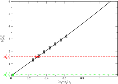
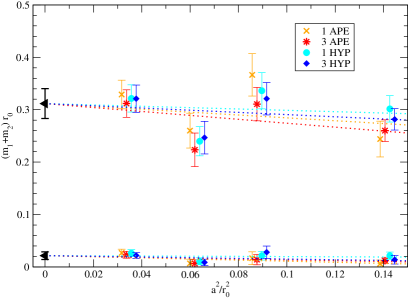
Figure 7: $M_{P}^{2}$ versus $m_{1}\!+\!m_{2}$ on our coarsest lattice (1 HYP operator) and the pertinent scaling plot for $2m_{ud}r_{0}$ and $(m_{ud}\!+\!m_{s})r_{0}$ (all filterings).

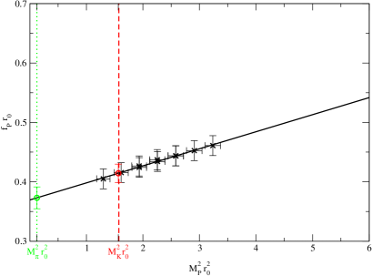
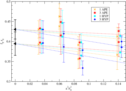
Figure 8: $f_{P}$ versus $M_{P}^{2}$ on our coarsest lattice (1 HYP) and the scaling plot for $f_{\pi}r_{0}$ and $f_{K}r_{0}$.

Given the promising localization properties of the filtered overlap, it is natural to ask whether this will lead to a better scaling behavior. There have been other scaling studies with the overlap action [20, 24, 25], but here we shall focus on the first continuum result for $m_{ud},m_{s}$ and $f_{\pi},f_{K}$ from quenched overlap data [26].

On the technical level, one more ingredient is needed, $Z_{S}\!=\!Z_{m}^{-1}$. We compute it with the RI-MOM method [27]. It turns out that the filtering leads to a rather mild $\beta$-dependence of the scalar renormalization factor, too [26].

For the scaling study we use 4 couplings, $\beta\!=\!5.66,5.76,5.84,6.0$, with lattice dimensions such as to have one matched spatial box size $L\!=\!1.5\,\mathrm{fm}$. We choose 4 quark masses, ranging from about ${1\over 3}m_{s}^{\mathrm{phys}}$ to $m_{s}^{\mathrm{phys}}$, and 4 filterings (1 APE, 3 APE, 1 HYP, 3 HYP). We do, however, not consider the unfiltered operator, simply because it is too demanding for our computational resources.

Fig. 7 shows the pseudoscalar mass squared versus the sum of the valence quark masses (the Sommer radius $r_{0}$ makes them dimensionless) on our coarsest lattice with the 1 HYP version of $D_{\mathrm{ov}}$. The analogous plots at the other couplings look rather similar (not shown). Imposing the physical value $M_{K}r_{0}\!=\!1.251$ yields a definition of $(m_{s}\!+\!m_{ud})r_{0}$ at this particular lattice spacing. Likewise, imposing $M_{\pi}r_{0}\!=\!0.3537$ yields $2m_{ud}r_{0}$ at this coupling. Repeating this procedure for the other operators and on the finer lattices, we are finally in a position to extrapolate to the continuum. We obtain the quenched continuum values

$$m_{s}^{\mathrm{\overline{MS}}}(2\,\mathrm{GeV})\! \!=\! \!119(10)(7)\,\mathrm{MeV}$$ (12)

$$m_{s}/m_{ud}\! \!=\! \!23.7(7.1)(4.5)$$ (13)

with the first error being statistical, the second systematic (up to quenching).

Fig. 8 shows the pseudoscalar decay constant versus the pseudoscalar mass squared, again on our coarsest lattice with the 1 HYP operator. Superimposing the data obtained with other filterings or at weaker coupling would reveal a rather good agreement. Using the same values for $M_{K}r_{0}$ and $M_{\pi}r_{0}$ as before, we get $f_{K}r_{0}$ and $f_{\pi}r_{0}$ at this coupling. Repeating this procedure on the finer lattices, we can extrapolate the pseudoscalar decay constants to the continuum. We obtain

$$f_{K}\! \!=\! \!170(10)(2)\,\mathrm{MeV}$$ (14)

$$f_{K}/f_{\pi}\! \!=\! \!1.17(4)(2)$$ (15)

in the continuum with a systematic uncertainty that does not include quenching effects.

Admittedly, our continuum extrapolations are somewhat courageous – we start from a lattice as coarse as $a^{-1}\!=\!1\,\mathrm{GeV}$ and have $a^{-1}\!=\!2\,\mathrm{GeV}$ on the finest one. Given this range and our statistical precision, we can only conjecture that we are in the Symanzik scaling regime. But in a strict sense this statement remains true with any statistical precision and any range of couplings.

It is interesting to compare our continuum results to those of [28]. The central values are consistent, but the relevant aspect is the error. The CP-PACS result was thought to be the “final” quenched value and consumed about half a year of runtime on their then new machine. Our calculation used an equivalent of less than 1 year on a stand-alone PC. And yet the net combined error (statistical and systematics, without quenching) is almost the same. This illustrates that the absence of additive mass renormalization, due to exact GW symmetry, has important practical consequences.

4 SUMMARY

The main features of overlap fermions with UV-filtering may be summarized as follows.

1. The overlap construction per se (with any undoubled kernel) brings a variety of invaluable conceptual features like on-shell chiral symmetry and a sound definition of the topological charge via the index theorem.

2. Using an UV-filtered Wilson kernel several technical advantages can be achieved: there is no need to tune the shift parameter $\rho$, the locality of the resulting $D_{\mathrm{ov}}$ and the normality of the kernel $D_{\mathrm{W},-\rho}$ are improved, furthermore $H_{\mathrm{W},-\rho}$ has a better condition number, and renormalization factors like $Z_{A}$ depend only weakly on the coupling.

3. The details of the filtering procedure seem rather irrelevant; one may use APE, HYP or stout-smearing with any set of parameters. The crucial issue from a conceptual viewpoint is that these parameters ($\alpha_{\mathrm{smear}}$ and $N_{\mathrm{iter}}$) are kept fixed when $\beta$ changes, just like the other parameter $\rho$ must stay fixed. In practice it seems advisable to stay with a moderate amount of filtering, e.g. 1 to 3 iterations with standard parameters.

4. Our exploratory scaling study suggests that such filtered overlap quarks enjoy good scaling properties already on rather coarse ($a^{-1}\simeq 1-1.5\,\mathrm{GeV}$) lattices. Under the proviso that more detailed studies with higher statistics confirm this finding, it seems conceivable that overlap quarks become the method of choice whenever high-precision results in the continuum are sought-for.

Acknowledgments: One of us (S.D.) likes to acknowledge useful discussions with Gian Carlo Rossi and Tony Kennedy during the workshop.

References

- [1] D.B. Kaplan, Phys. Lett. B 288, 342 (1992) [hep-lat/9206013]. V. Furman and Y. Shamir, Nucl. Phys. B 439, 54 (1995) [hep-lat/9405004]. Y. Shamir, Nucl. Phys. B 406, 90 (1993) [hep-lat/9303005].
- [2] H. Neuberger, Phys. Lett. B 417, 141 (1998) [hep-lat/9707022]. H. Neuberger, Phys. Lett. B 427, 353 (1998) [hep-lat/9801031].
- [3] P. Hasenfratz, Nucl. Phys. B 525, 401 (1998) [hep-lat/9802007].
- [4] P.H. Ginsparg and K.G. Wilson, Phys. Rev. D 25, 2649 (1982).
- [5] P. Hasenfratz, V. Laliena and F. Niedermayer, Phys. Lett. B 427, 125 (1998) [hep-lat/9801021]. F. Niedermayer, Nucl. Phys. Proc. Suppl. 73, 105 (1999) [hep-lat/9810026].
- [6] M. Lüscher, Phys. Lett. B 428, 342 (1998) [hep-lat/9802011].
- [7] S. Capitani, M. Göckeler, R. Horsley, P.E.L. Rakow and G. Schierholz, Phys. Lett. B 468, 150 (1999) [hep-lat/9908029].
- [8] W. Bietenholz, Eur. Phys. J. C 6, 537 (1999) [hep-lat/9803023]. W. Bietenholz and I. Hip, Nucl. Phys. B 570, 423 (2000) [hep-lat/9902019]. W. Bietenholz, hep-lat/0007017. C. Gattringer, I. Hip and C.B. Lang, Nucl. Phys. B 597, 451 (2001) [hep-lat/0007042]. T. DeGrand [MILC Collab.], Phys. Rev. D 63, 034503 (2001) [hep-lat/0007046].
- [9] T. Blum et al., Phys. Rev. D 55, 1133 (1997) [hep-lat/9609036]. K. Orginos, D. Toussaint and R.L. Sugar [MILC Collab.], Phys. Rev. D 60, 054503 (1999) [hep-lat/9903032].
- [10] A. Hasenfratz and F. Knechtli, Phys. Rev. D 64, 034504 (2001) [hep-lat/0103029].
- [11] J.M. Zanotti et al. [CSSM Collab.], Phys. Rev. D 65, 074507 (2002) [hep-lat/0110216]. T. DeGrand, A. Hasenfratz and T.G. Kovacs, Phys. Rev. D 67, 054501 (2003) [hep-lat/0211006].
- [12] T.G. Kovács, hep-lat/0111021. T.G. Kovács, Phys. Rev. D 67, 094501 (2003) [hep-lat/0209125]. W. Kamleh, D.H. Adams, D.B. Leinweber and A.G. Williams, Phys. Rev. D 66, 014501 (2002) [hep-lat/0112041]. S. Dürr, C. Hoelbling and U. Wenger, Phys. Rev. D 70, 094502 (2004) [hep-lat/0406027].
- [13] M. Albanese et al. [APE Collab.], Phys. Lett. B 192, 163 (1987).
- [14] C. Morningstar and M.J. Peardon, Phys. Rev. D 69, 054501 (2004) [hep-lat/0311018].
- [15] S. Dürr, C. Hoelbling and U. Wenger, JHEP 0509, 030 (2005) [hep-lat/0506027].
- [16] P. Hernandez, K. Jansen and L. Lellouch, hep-lat/0001008.
- [17] M. Golterman and Y. Shamir, Phys. Rev. D 68, 074501 (2003) [hep-lat/0306002]. M. Golterman, Y. Shamir and B. Svetitsky, Phys. Rev. D 71, 071502 (2005) [hep-lat/0407021]. M. Golterman, Y. Shamir and B. Svetitsky, Phys. Rev. D 72, 034501 (2005) [hep-lat/0503037].
- [18] P. Hernandez, K. Jansen and M. Lüscher, Nucl. Phys. B 552, 363 (1999) [hep-lat/9808010].
- [19] S. Dürr, C. Hoelbling and U. Wenger, hep-lat/0509111.
- [20] J. Wennekers and H. Wittig, hep-lat/0507026.
- [21] T. DeGrand, Phys. Rev. D 67, 014507 (2003) [hep-lat/0210028].
- [22] Z. Fodor, S.D. Katz and K.K. Szabo, JHEP 0408, 003 (2004) [hep-lat/0311010]. G.I. Egri, Z. Fodor, S.D. Katz and K.K. Szabo, hep-lat/0510117. T. DeGrand and S. Schaefer, Phys. Rev. D 71, 034507 (2005) [hep-lat/0412005]. T. DeGrand and S. Schaefer, Phys. Rev. D 72, 054503 (2005) [hep-lat/0506021]. N. Cundy et al., hep-lat/0502007.
- [23] R.C. Brower, H. Neff and K. Orginos, hep-lat/0511031.
- [24] S. Dürr and C. Hoelbling, Phys. Rev. D 69, 034503 (2004) [hep-lat/0311002]. S. Dürr and C. Hoelbling, Phys. Rev. D 71, 054501 (2005) [hep-lat/0411022].
- [25] S.J. Dong, F.X. Lee, K.F. Liu and J.B. Zhang, Phys. Rev. Lett. 85, 5051 (2000) [hep-lat/0006004]. C. Gattringer, P. Huber and C.B. Lang, hep-lat/0509003. R. Babich et al., hep-lat/0509027. T. Draper et al., hep-lat/0510075.
- [26] S. Dürr and C. Hoelbling, Phys. Rev. D 72, 071501 (2005) [hep-ph/0508085].
- [27] G. Martinelli, C. Pittori, C.T. Sachrajda, M. Testa and A. Vladikas, Nucl. Phys. B 445, 81 (1995) [hep-lat/9411010].
- [28] S. Aoki et al. [CP-PACS Collab.], Phys. Rev. D 67, 034503 (2003) [hep-lat/0206009].