Infrared Gluon Propagator from lattice QCD: results from large asymmetric lattices

Abstract

The infrared limit of the lattice Landau gauge gluon propagator is studied. We show that the lattice data is compatible with the pure power law $(q^{2})^{2\kappa}$ solution of the Dyson-Schwinger equations. Using various lattice volumes, the infinite volume limit for the exponent $\kappa$ is measured. Although, the results allow $\kappa=0.498-0.525$, the lattice data favours $\kappa\sim 0.52$, which would imply a vanishing zero momentum gluon propagator.

1 Introduction and motivation

The gluon propagator is a fundamental Green’s function of Quantum Chromodynamics (QCD). Certainly, a good description of this two point function is required to understand the non-perturbative regime of the theory. Moreover, in the Landau gauge, the gluon and the ghost propagators at zero momentum are connected with possible confinement mechanisms. In particular, the Kugo-Ojima confinement mechanism requires an infinite zero momentum ghost propagator [1, 2] and the Zwanziger horizon condition [3, 4, 5] implies either reflection positivity violation or a null zero momentum gluon propagator. From this last condition it can be proved that the zero momentum ghost propagator should diverge [6].

The computation of the gluon and ghost propagators for the full range of momenta cannot be done in perturbation theory. Presently, we have to rely either on Dyson-Schwinger equations (DSE) or on the lattice formulation of QCD; both are first principles approaches. In the first technique a truncation of an infinite tower of equations, together with the parametrizations of a number of vertices, namely the three gluon and the gluon-ghost vertices, is required to solve the equations. In the second, one has to care about finite volume and finite lattice spacing effects. Hopefully, the two solutions will be able to reproduce the same solution. In this article we are concerned with the lattice Landau gauge gluon propagator in momentum space,

$$D^{ab}_{\mu\nu}(q)~{}=~{}\delta^{ab}\,\left(\delta_{\mu\nu}\,-\,\frac{q_{\mu}q_{\nu}}{q^{2}}\right)\,\frac{Z(q^{2})}{q^{2}}\,,$$ (1)

for pure gauge theory. The form factor $Z(q^{2})$ is the gluon dressing function.

Recently, in [7] the DSE were solved for the gluon and ghost propagators in the deep infrared region. The solution assumes ghost dominance and is a pure power law [8], with the exponents of the two propagators related by a single number $\kappa$. For the gluon dressing function, the solution reads

$$Z(q^{2})~{}=~{}z\left(q^{2}\right)^{2\kappa}\,.$$ (2)

The DSE equations allow a determination of the exponent $\kappa=0.595$, which, for the zero momentum, implies a null (infinite) gluon (ghost) propagator, in agreement with the criteria described above, and a finite strong coupling constant defined from the gluon and ghost dressing functions [11, 12]. Renormalization group analysis based on the flow equation [13, 14, 15] were able to predict, for the solution (2), the range of possible values for the exponent. The results of this analysis being $0.52\,\leq\,\kappa\,\leq\,0.595$, implying, again, a null (infinite) zero momentum gluon (ghost) propagator. A similar analysis of the DSE but using time-independent stochastic quantisation [16, 17] predicted the same behaviour and $\kappa=0.52145$.

The reader should be aware that not all solutions of the DSE predict a vanishing zero momentum gluon propagator. In [18, 19], the authors computed a solution of the DSE with a finite zero momentum gluon propagator. Moreover, in [20, 21] it was claimed that the gluon and ghost propagators in the deep infrared region are not connected via the same exponent $\kappa$ and that there isn’t yet a clear theoretical answer concerning the value of zero momentum gluon propagator. According to the authors, the range of possible values goes from zero to infinity.

On the lattice, there are a number of studies concerned with the gluon propagator [22, 23, 24, 25, 26, 27]. On large lattices, the propagator was investigated in [28]. Although the lattices used had a limited access to the deep infrared region, the authors conclude in favour of a finite zero momentum gluon propagator, which would imply $\kappa=0.5$ for the solution (2). In [29], the infinite volume and continuum limits of the Landau gauge gluon propagator were investigated using various lattices and, again, the data supported a finite zero momentum gluon propagator. In [24], the three-dimensional lattice SU(2) Landau gauge propagator was studied with the authors measuring an infrared exponent compatible with the corresponding DSE solution.

In order to access the deep infrared region, in [30, 31, 32] we have computed the gluon propagator with large asymmetric lattices. The fits to (2) produced always $\kappa<0.5$. However, the inclusion of corrections to the leading behaviour given by (2) or when the gluon dressing function was modelled, either in the momenta region $q<1$ GeV or for all the momenta, $\kappa$ becomes larger than 0.5. Moreover, in the preliminary finite volume study [32, 34] of the two point gluon function it came out that $\kappa$ increases with the lattice volume and, in that sense, previously computed values should be regarded as lower bounds. The previous studies do not provide a clear answer about the zero momentum gluon propagator. In this paper, we update the results of our previous publications for the infrared region, using a larger set of lattices, that allows a better control of the infinite volume extrapolation. Two different extrapolations to the infinite volume are performed, namely the extrapolation of $\kappa$ and the extrapolation of the propagator, giving essentially the same result. The main conclusions from this investigation being that the lattice data is compatible with the DSE solution (2) for the infrared gluon dressing function, for momenta $\sim 150$ MeV or lower, and that the infinite volume extrapolation of the lattice gluon propagator seems to favour a vanishing zero momentum gluon propagator.

2 Field Definitions and Notation

In the lattice formulation of QCD, the gluon fields $A^{a}_{\mu}$ are replaced by the links

$$U_{\mu}(x)~{}=~{}e^{iag_{0}A_{\mu}(x+a\hat{e}_{\mu}/2)}~{}+~{}\mathcal{O}(a^{3})~{}~{}~{}\in~{}SU(3)\,,$$ (3)

where $\hat{e}_{\mu}$ are unit vectors along $\mu$ direction. QCD is a gauge theory, therefore the fields related by gauge transformations

$$U_{\mu}(x)~{}\longrightarrow~{}g(x)~{}U_{\mu}(x)~{}g^{\dagger}(x+a\hat{e}_{\mu})\,,\hskip 28.45274ptg\in SU(3)\,,$$ (4)

are physically equivalent. The set of links related by gauge transformations to $U_{\mu}(x)$ is the gauge orbit of $U_{\mu}(x)$.

The gluon field associated to a gauge configuration is given by

$$A_{\mu}(x+a\hat{e}_{\mu}/2)~{}=~{}\frac{1}{2ig_{0}}\Big{[}U_{\mu}(x)-U^{\dagger}_{\mu}(x)\Big{]}~{}-~{}\frac{1}{6ig_{0}}\mbox{Tr}\Big{[}U_{\mu}(x)-U^{\dagger}_{\mu}(x)\Big{]}$$ (5)

up to corrections of order $a^{2}$.

On the lattice, due to the periodic boundary conditions, the discrete momenta available are

$$\hat{q}_{\mu}~{}=~{}\frac{2\pi n_{\mu}}{aL_{\mu}}\,,\hskip 14.22636ptn_{\mu}~{}=~{}0,\,1,\,\dots\,L_{\mu}-1\,,$$ (6)

where $L_{\mu}$ is the lattice length over direction $\mu$. The momentum space link is

$$U_{\mu}(\hat{q})~{}=~{}\sum\limits_{x}~{}e^{-i\hat{q}x}~{}U_{\mu}(x)$$ (7)

and the momentum space gluon field

$$A_{\mu}(\hat{q}) = \sum\limits_{x}~{}e^{-i\hat{q}\left(x+a\hat{e}_{\mu}/2\right)}~{}A_{\mu}(x+a\hat{e}_{\mu}/2)$$ (8)

$$= \frac{e^{-i\hat{q}_{\mu}a/2}}{2ig_{0}}\Bigg{\{}~{}\Big{[}U_{\mu}(\hat{q})-U^{\dagger}_{\mu}(-\hat{q})\Big{]}\,-\,\frac{1}{3}\mbox{Tr}\Big{[}U_{\mu}(\hat{q})-U^{\dagger}_{\mu}(-\hat{q})\Big{]}~{}\Bigg{\}}~{}.$$

The gluon propagator is the gluon two point correlation function. The dimensionless lattice two point function is

$$\langle A^{a}_{\mu}(\hat{q})~{}A^{b}_{\nu}(\hat{q}^{\prime})\rangle~{}=~{}D^{ab}_{\mu\nu}(\hat{q})~{}V~{}\delta(\hat{q}+\hat{q}^{\prime})~{}.$$ (9)

On the continuum, the momentum space propagator in the Landau gauge is given by

$$D^{ab}_{\mu\nu}(\hat{q})~{}=~{}\delta^{ab}~{}\Big{(}\delta_{\mu\nu}~{}-~{}\frac{q_{\mu}q_{\nu}}{q^{2}}\Big{)}~{}D(q^{2})~{}.$$ (10)

Assuming that the deviations from the continuum are negligable, the lattice scalar function $D(q^{2})$ can be computed directly from (10) as follows

$$D(q^{2})~{}=~{}\frac{2}{(N^{2}_{c}-1)(N_{d}-1)V}\sum\limits_{\mu}~{}\langle~{}\mbox{Tr}\left[A_{\mu}(\hat{q})\,A_{\mu}(-\hat{q})\right]~{}\rangle\,,\hskip 8.5359ptq\neq 0\,,$$ (11)

and

$$D(0)~{}=~{}\frac{2}{(N^{2}_{c}-1)N_{d}V}\sum\limits_{\mu}~{}\langle~{}\mbox{Tr}\left[A_{\mu}(\hat{q})\,A_{\mu}(-\hat{q})\right]~{}\rangle\,,\hskip 8.5359ptq=0\,,$$ (12)

where

$$q_{\mu}\,=\,\frac{2}{a}~{}\sin\Big{(}\frac{\hat{q}_{\mu}a}{2}\Big{)}\,,$$ (13)

$N_{c}=3$ is the dimension of the group, $N_{d}=4$ the number of spacetime dimensions and $V$ is the lattice volume.

3 The Landau Gauge

On the continuum, the Landau gauge is defined by

$$\partial_{\mu}A_{\mu}~{}=~{}0\,.$$ (14)

This condition defines the hyperplane of transverse configurations

$$\Gamma~{}\equiv~{}\{A:~{}\partial\cdot A\,=\,0\}~{}.$$ (15)

It is well known [35] that $\Gamma$ includes more than one configuration from each gauge orbit. In order to try to solve the problem of the nonperturbative gauge fixing, Gribov suggested the use of additional conditions, namely the restriction of physical configurational space to the region

$$\Omega~{}\equiv~{}\{A:~{}\partial\cdot A\,=\,0,~{}\textit{M}[A]\,\geq\,0\}~{}\subset~{}\Gamma\,,$$ (16)

where $\textit{M}[A]~{}\equiv~{}-\nabla\cdot D[A]$ is the Faddeev-Popov operator. However, $\Omega$ is not free of Gribov copies and does not provide a proper definition of physical configurations.

A suitable definition of the physical configurational space is given by the fundamental modular region $\Lambda\subset\Omega$, the set of the absolute minima of the functional

$$F_{A}[g]~{}=~{}\int d^{4}x~{}\sum_{\mu}~{}\mbox{Tr}\left[A_{\mu}^{g}(x)A_{\mu}^{g}(x)\right]\,.$$ (17)

In this article, the problem of Gribov copies on the computation of the gluon propagator will not be discussed. For a numerical study on Gribov copies see [36, 37] and references therein.

On the lattice, the situation is similar to the continuum theory. The Landau gauge is defined by maximising the functional

$$F_{U}[g]~{}=~{}C_{F}\sum_{x,\mu}\,\mbox{Re}\,\{\,\mbox{Tr}\,[g(x)U_{\mu}(x)g^{\dagger}(x+\hat{\mu})]\,\}$$ (18)

where

$$C_{F}~{}=~{}\frac{1}{N_{d}N_{c}V}$$ (19)

is a normalization constant. Let $U_{\mu}$ be the configuration that maximises $F_{U}[g]$ on a given gauge orbit. For configurations near $U_{\mu}$ on its gauge orbit, we have

$$F_{U}[1+i\omega(x)]=F_{U}[1]+\frac{C_{F}}{4}\sum_{x,\mu}i\omega^{a}(x)\mbox{Tr}\Big{[} \lambda^{a}\left(U_{\mu}(x)\,-\,U_{\mu}(x-\hat{\mu})\right)~{}-$$ (20)

$$\lambda^{a}\left(U^{\dagger}_{\mu}(x)\,-\,U^{\dagger}_{\mu}(x-\hat{\mu})\right)\Big{]}\,,$$

where $\lambda^{a}$ are the Gell-Mann matrices. By definition, $U_{\mu}$ is a stationary point of $F$, therefore

$$\frac{\partial F}{\partial\omega^{a}(x)}~{}=~{}\frac{i\,C_{F}}{4}\sum_{\mu}\mbox{Tr}\Big{[} \lambda^{a}\left(U_{\mu}(x)\,-\,U_{\mu}(x-\hat{\mu})\right)~{}-$$ (21)

$$\lambda^{a}\left(U^{\dagger}_{\mu}(x)\,-\,U^{\dagger}_{\mu}(x-\hat{\mu})\right)\Big{]}~{}=~{}0\,.$$

In terms of the gluon field, this condition reads

$$\sum_{\mu}\mbox{Tr}\Big{[}~{}\lambda^{a}\left(A_{\mu}(x+a\hat{\mu}/2)-A_{\mu}(x-a\hat{\mu}/2)\right)~{}\Big{]}\,+\,\mathcal{O}(a^{2})~{}=~{}0\,,$$ (22)

or

$$\sum_{\mu}\partial_{\mu}A^{a}_{\mu}(x)~{}+~{}\mathcal{O}(a)~{}=~{}0\,,$$ (23)

i.e. (21) is the lattice equivalent of the continuum Landau gauge condition. The lattice Faddeev-Popov operator $M(U)$ is given by the second derivative of (18).

Similarly to the continuum theory, on the lattice one defines the region of stationary points of (18)

$$\Gamma~{}\equiv~{}\{U:~{}\partial\cdot A(U)\,=\,0\}\,,$$ (24)

the Gribov’s region $\Omega$ of the maxima of (18),

$$\Omega~{}\equiv~{}\{U:~{}\partial\cdot A(U)=0~{}\mbox{and}~{}M(U)\geq 0\}$$ (25)

and the fundamental modular region $\Lambda$ defined as the set of the absolute maxima of (18). A proper definition of the lattice Landau gauge chooses from each gauge orbit, the configuration belonging to the interior of $\Lambda$.

In this work, the gauge fixing algorithm used is a Fourier accelerated steepest descent method (SD) as defined in [40]. In each iteration, the algorithm chooses

$$g(x)\,=\,\exp\Bigg{[}\hat{F}^{-1}\,\frac{\alpha}{2}\,\frac{p_{max}^{2}a^{2}}{p^{2}a^{2}}\,\hat{F}\,\left(\sum_{\nu}\Delta_{-\nu}\left[U_{\nu}(x)\,-\,U^{\dagger}_{\nu}(x)\right]\,-\,\mbox{trace}\right)\Bigg{]}$$ (26)

where

$$\Delta_{-\nu}\left(U_{\mu}(x)\right)~{}=~{}U_{\mu}(x-a\hat{e}_{\nu})\,-\,U_{\mu}(x)\,,$$ (27)

$p^{2}$ are the eigenvalues of $(-\partial^{2})$, $a$ is the lattice spacing and $\hat{F}$ represents a fast Fourier transform (FFT). For numerical purposes, it is enough to expand to first order the exponential in (26), followed by a reunitarization of $g(x)$. On the gauge fixing process, the quality of the gauge fixing is measured by

$$\theta~{}=~{}\frac{1}{VN_{c}}~{}\sum_{x}\mbox{Tr}[\Delta(x)\Delta^{{\dagger}}(x)]$$ (28)

where

$$\Delta(x)~{}=~{}\sum_{\nu}\left[U_{\nu}(x-a\hat{e}_{\nu})\,-\,U^{\dagger}_{\nu}(x)\,-\,\mbox{h.c.}\,-\,\mbox{trace}\right]$$ (29)

is the lattice version of $\partial_{\mu}A_{\mu}\,=\,0$.

4 Lattice setup

Lattice	Update	therm.	Sep.	Conf
$8^{3}\times 256$	7OVR+4HB	1500	1000	80
$10^{3}\times 256$	7OVR+4HB	1500	1000	80
$12^{3}\times 256$	7OVR+4HB	1500	1000	80
$14^{3}\times 256$	7OVR+4HB	3000	1000	80
$16^{3}\times 256$	7OVR+4HB	3000	1500	155
$18^{3}\times 256$	7OVR+4HB	3000	1500	40

Table 1: Lattice setup used in the study of the gluon propagator volume dependence.

The gluon propagator was computed using the SU(3) pure gauge, Wilson action, $\beta=6.0$ configurations for the lattices reported in table 1. All configurations were generated with the MILC code http://physics.indiana.edu/~sg/milc.html. The table describes the combined overrelaxed+heat bath Monte Carlo sweeps, the number of thermalisation sweeps of the combined overrelaxed+heat bath steps, the number of combined sweeps separating each configuration and the total number of configurations for each lattice. The statistical errors on the propagators were computed using the jackknife method.

The propagators computed in this study have finite volume effects [32]. An example is seen in figure 1 where the bare gluon propagator, $D(q^{2})=Z(q^{2})/q^{2}$, is plotted for temporal momenta $q_{t}$ and spatial momenta $q_{x}$ for the smallest and largest lattices. Figure 2 shows $D(q^{2})$ for temporal $q\leq 1$ GeV for the volumes considered in this study, including the two lattices $16^{3}\times 48$ and $32^{3}\times 64$, $\beta=6.0$, temporal momenta propagators from [28]. For the lattices discussed here, it was observed that the difference between the propagators computed using only pure temporal or pure spatial momenta becames smaller as the spatial extension of the lattice increases. Moreover, the differences vanish for sufficient high momenta and become larger for smaller momenta. Furthermore, it was observed that, for the smallest momenta, the propagator decreases as the lattice volume increases, in agreement with what was observed in previous studies of the volume dependence [29, 32]. In this work, we will not discuss what should be the right choice of momenta to minimize finite volume effects. Since our smallest momenta are pure temporal momenta, the results of the various lattices will be combined to investigate the volume dependence of the infrared gluon propagator. In the following and in order to access the infrared region, only the pure temporal momenta will be considered.

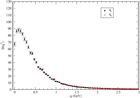
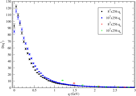
Figure 1: Bare gluon dressing function for all momenta for the largest (top) and the two smallest (bottom) lattices. The figure shows the gluon propagator computed with pure temporal momenta $q_{t}$ and pure spatial momenta $q_{x}$. For the spatial momenta a $Z_{3}$ average was performed.

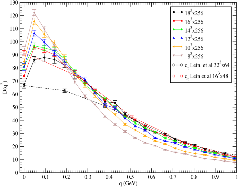
Figure 2: Bare gluon dressing function for temporal momenta for all lattices volumes. For comparisation, the figure includes the $16^{3}\times 48$ and $32^{3}\times 64$ propagators computed at $\beta=6.0$ in [28].

5 The Infrared Gluon Dressing Function

Lattice	$z(q^{2})^{2\kappa}$		$z(q^{2})^{2\kappa}(1+aq^{2})$		$z(q^{2})^{2\kappa}(1+aq^{2}+bq^{4})$
$8^{3}\times 256$	$0.4496^{+22}_{-29}$	2.14	$0.4773^{+37}_{-52}$	0.02	$0.4827^{+75}_{-74}$	0.00
$10^{3}\times 256$	$0.4650^{+31}_{-37}$	0.10	$0.4827^{+49}_{-68}$	0.25	$0.4765^{+104}_{-99}$	0.14
$12^{3}\times 256$	$0.4663^{+30}_{-36}$	1.19	$0.4822^{+51}_{-69}$	0.21	$0.4849^{+94}_{-97}$	0.18
$14^{3}\times 256$	$0.4918^{+26}_{-40}$	0.09	$0.5053^{+52}_{-67}$	0.16	$0.4992^{+100}_{-80}$	0.06
$16^{3}\times 256$	$0.4859^{+22}_{-24}$	0.40	$0.5070^{+36}_{-50}$	0.44	$0.5131^{+67}_{-64}$	1.03
$18^{3}\times 256$	$0.5017^{+49}_{-40}$	0.20	$0.5169^{+89}_{-70}$	0.00	$0.514^{+12}_{-15}$	0.00

Table 2: $\kappa$ and $\chi^{2}/d.o.f.$ from fitting the different lattices. In all fits, the range of momenta considered starts with the lowest non-vanishing momentum. The errors shown are statistical and were computed using the bootstrap method, with the number of bootstrap samples being about ten times the number of configurations. For the momenta range considered in the fits, the correction associated with $aq^{2}$ and $aq^{2}+bq^{4}$ to the pure power law are below 20% and 30%, respectively. For the smallest lattice, the corrections are larger. However, this lattice is never used in the extrapolations.

An analytical solution of the DSE for the gluon dressing function is given by (2). For $\beta=6.0$, the lattice spacing is $a^{-1}=1.94(5)$ GeV [33], therefore our smallest nonzero momentum is $47.6\pm 1.2$ MeV. Since we do not know at what momenta the above solution sets in, besides the pure power law, we will consider also polynomial corrections to the leading behaviour, i.e.

$$Z(q^{2})~{}=~{}z\,\left(q^{2}\right)^{2\kappa}\,\left\{1~{}+\sum_{n}a_{n}\left(q^{2}\right)^{n}\right\}\,,$$ (30)

with $n=1$, $2$. In order to be as close as possible to the infrared region, in all fits only the smallest range of momenta will be considered, i.e. all reported fits have one degree of freedom. The $\kappa$ and $\chi^{2}/d.o.f.$ for the various fits are given in table 2. In general, the data is well described by any of the above functions. The exception being the smallest lattice for a pure power law. $\kappa$ shows finite volume effects, becoming larger for larger volumes. Note that for the largest lattices, the various $\kappa$ computed with the corrections to the pure power law agree within one standard deviation. Moreover, for the largest lattice, the various $\kappa$ agree with each other within less than 1.5 standard deviations. Figure 3 shows the results of the fits to $\kappa$ as function of the inverse of the lattice volume.

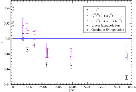
Figure 3: $\kappa$ as a function of the inverse volume. Note that in order to make the plot more clear, the $\kappa$ from the fits to the corrections to the pure power law were shifted in the $1/V$ axis.

The infinite volume $\kappa$ can be estimated combining the results of table 2. Assuming, for each of the reported fits to the dressing function, either a linear or a quadratic dependence on $1/V$ for $\kappa(V)$ and excluding the smallest lattice, it comes out that the figures on the first column, the pure power law, are not described by any of these functional forms. Figure 3 includes, besides the $\kappa$ values for each volume, the extrapolated $\kappa$ from fitting $\kappa(1/V)$ to a linear or quadratic function of $1/V$. Note that the points are computed independently for each of the corrections to the pure power law considered. The extrapolated $\kappa$ agree within one standard deviation, with the quadratic fits to $\kappa(1/V)$ giving larger errors and lying above the linear fits. For the linear extrapolation the results give

$$\kappa_{\infty}~{}=~{}0.5167(55)\,,\hskip 19.91684pt\kappa_{\infty}~{}=~{}0.5218(80)$$ (31)

when the extrapolation uses the data from the quadratic or the quartic corrections to (2). The corresponding $\chi^{2}/d.o.f.$ being 1.44 and 0.49. For the quadratic fit the extrapolated values are

$$\kappa_{\infty}~{}=~{}0.537(13)\,,\hskip 19.91684pt\kappa_{\infty}~{}=~{}0.541(20)\,;$$ (32)

the $\chi^{2}/d.o.f.$ being 0.72 and 0.10, respectively. The errors $\kappa$ were computed assuming gaussian error propagation. The results of the extrapolation to the infinite lattice volume, point to a value of $\kappa$ in the range $0.51-0.56$.

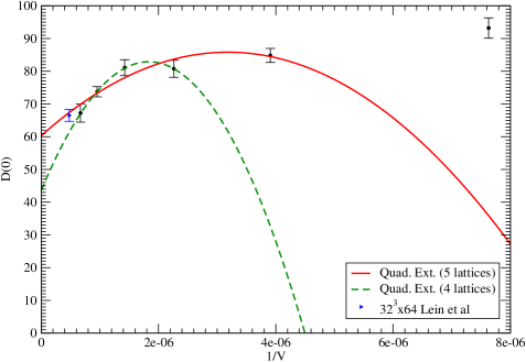
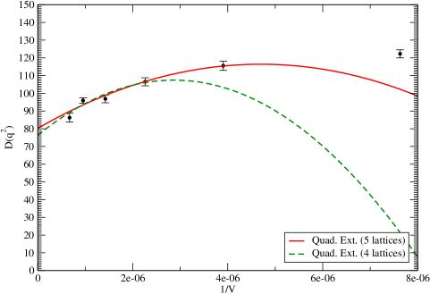
Figure 4: Bare gluon propagator for the two smallest momenta as a function of the inverse volume. For comparison, for zero momentum we include $D(0)$ from the largest lattice of [28], i.e. $32^{3}\times 64$.

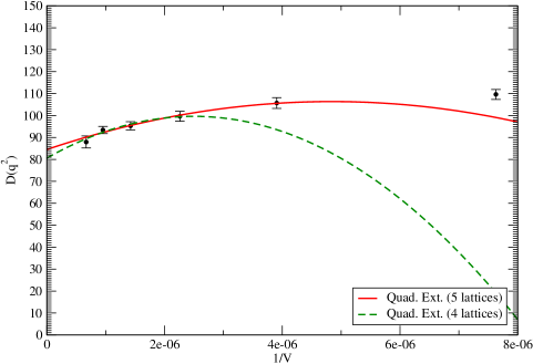
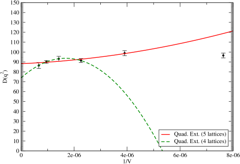
Figure 5: Bare gluon propagator as a function of the inverse volume for the third and fourth smallest momenta.

So far we have extrapolated the $\kappa$ values. Alternatively, one can extrapolate directly the gluon propagator and fit the associated dressing function. In figures 4 and 5 the bare propagator is plotted, as function of the volume, for the lowest four momenta. For all these momenta, we tried linear, quadratic, cubic and quartic extrapolations. In table 3 the $\chi^{2}/d.o.f.$ is reported for the various extrapolations considered and for the lowest four momenta.

$p$	Set I				Set II			Set III
	$8^{3}-18^{3}\times 256$				$10^{3}-18^{3}\times 256$			$12^{3}-18^{3}\times 256$
	Lin	Quad	Cub	Quart	Lin	Quad	Cub	Lin	Quad
0	2.84	2.60	1.54	0.21	3.08	1.94	0.13	2.99	0.01
1	6.15	1.95	2.60	4.53	2.66	2.67	4.71	2.92	5.07
2	2.02	0.44	0.56	0.71	0.68	0.59	0.77	0.72	0.90
3	1.66	1.02	1.32	0.06	0.85	1.20	0.03	1.04	0.00

Table 3: The $\chi^{2}/d.o.f.$ for the extrapolations to the infinite volume of the four lowest momenta gluon propagator assuming a linear (Lin), quadratic (Quad), cubic (Cub) and quartic (Quart) polinomial dependence on $1/V$ and for various sets of data.

In the following, we will not consider extrapolations using all lattices (set I), because it involves our smallest lattice, which is too short $\sim 0.8$ fm in the spatial directions. Note, however, that the data reported in table 3 point towards a smooth approach to the infinite volume limit, starting from lattices sizes as small as 0.8 fm. Furthermore, figures 4 and 5 suggest that we should not use a linear extrapolation. According to the figures, a quadratic extrapolation, or a higher power of the inverse volume, seems to be more suitable. However, for set II, and for the first non-vanishing momentum, the cubic extrapolation gives a quite poor description of the data, when compared to the quadratic fit. So, for the reasons explained above, from now on we will consider only the quadratic extrapolation using set II and III.

Figures 4 and 5 show the lattice data together with the two quadratic extrapolations to the infinite volume. Note that in both extrapolations, the worst $\chi^{2}/d.o.f.$ is associated with the first nonzero momentum. Indeed, as can be seen in figure 4, for this momentum the data seems to fluctuate more than for the other momenta. For larger momenta the behaviour of the gluon propagator as a function of the volume becomes smoother.

In [29] the infinite volume of the renormalized zero momentum gluon propagator was computed. The chosen renormalization condition was

$$\left.D_{R}(q^{2})\right|_{q^{2}=\mu^{2}}~{}=~{}\frac{1}{\mu^{2}}\,;$$ (33)

the lattice data was renormalized at $\mu=4$ GeV. The quoted extrapolated renormalized zero momentum gluon propagator being $7.95(13)$ GeV^-2. Our largest momentum available is $q=3.88$ GeV, a slightly lower value. Performing the renormalization in the same way but at the scale $\mu=3.88$ GeV, it comes

$$D_{R}(0)~{}=~{}\left\{\begin{array}[]{rcl}6.3\pm 1.4~{}\mbox{GeV}^{-2}&&\mbox{set III data,}\\ 10.9\pm 0.8~{}\mbox{GeV}^{-2}&&\mbox{set II data.}\end{array}\right.$$ (34)

The quoted errors are pure statistical. The value quoted in [29] is in between the above figures, with the result from the so called set III being almost compatible within one standard deviation with $7.95(13)$ GeV^-2 and the result from set II being compatible only at three standard deviations.

The extrapolated propagators can be seen in figure 6; the errors were computed assuming gaussian error propagation. For infrared momenta, the extrapolated propagators interpolate between the two lattices simulated in [28]. Moreover, for zero momentum the extrapolated propagators are smaller than the propagator of Leinweber et al computed with their largest lattice. The extrapolated propagators from fitting the two different sets of lattices are compatible, at least, at the level of two standard deviations. The propagator computed from set III shows much larger statistical errors. The differences between the two propagators are larger for smaller momenta. This difference can be used to estimate systematic errors.

The fit of the dressing function computed from the extrapolated propagator, obtained from set II, to the first three nonzero momenta to the pure power law gives $\kappa=0.5215(29)$ and has a $\chi^{2}/d.o.f.=0.02$. Similar fits but using the corrections to (2) produce larger values for the same exponent ($\sim 0.55$). All the computed $\kappa$’s are compatible with a vanishing zero momentum gluon propagator. Moreover, the fit to the pure power law produces a number which agrees well with the estimation from an extrapolation on $\kappa$ - see equations (31) and (32). If, instead, we perform the same analysis but for the extrapolated propagator obtained from set III, then $\kappa=0.4979(66)$ and $\chi^{2}/d.o.f.=0.27$. Again, the fits with corrections to the pure power law give large values for $\kappa=0.52-0.53$. Note that now the $\kappa$ fitting the pure power law is smaller than the corresponding value obtained from our largest lattice (see table 2) and is compatible with $\kappa=0.5215(29)$ within two and a half standard deviations.

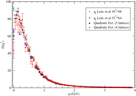
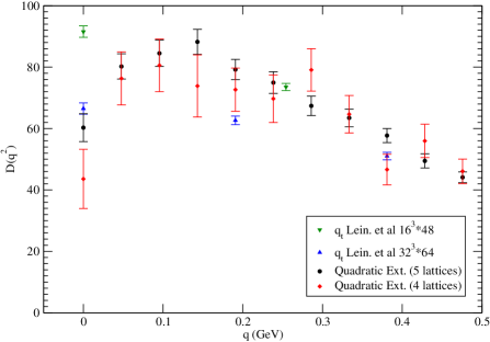
Figure 6: The bare extrapolated gluon propagator. The full range of temporal momenta is seen on the top with a zoom for the infrared region on the bottom. The errors on the propagator were computed assuming a gaussian error propagation. For comparisation, the figure includes the $16^{3}\times 48$ and $32^{3}\times 64$ propagators computed at $\beta=6.0$ in [28].

6 Results and Conclusion

We have computed the Landau gauge gluon propagator for large asymmetric lattices with different volumes. For each volume, we have checked that the lattice dressing function is well described by the DSE solution (2) for momenta below $\sim 150$ MeV by fitting the above functional form. The exception being our smallest lattice $8^{3}\times 256$. Note that in all these fits $Z(q^{2})|_{q=0}$ was never used. In what concerns the infrared exponent $\kappa$, the data shows finite volume effects, with $\kappa$ becoming larger for larger volumes. In this sense, all values in table 2 can be read as lower bounds on the infinite volume figure.

The infinite volume $\kappa$ was estimated in two different ways: i) from an extrapolation of the values reported in table 2, assuming a linear and a quadratic dependence on the inverse volume; ii) extrapolating the propagator, assuming a quadratic dependence on $1/V$. The results of the first method are (31), (32), giving an weighted mean value of $\kappa=0.5246(46)$. The value for the exponent from extrapolating directly the gluon propagator being $\kappa=0.5215(29)$, if one considers the five largest lattices (set II), and $\kappa=0.4979(66)$, if one considers the four largest lattices (set III). The first value is on the top of the value obtained from extrapolating directly $\kappa$ as function of the volume. Moreover, these two values agree well with the time-independent stochastic quantisation prediction $\kappa=0.52145$ [16, 17] and are within the range of possible values estimated with renormalization group arguments [13, 14, 15], $0.52\,\leq\,\kappa\,\leq\,0.595$. All these results point towards a vanishing zero momentum gluon propagator. The $\kappa=0.4979(66)$, obtained from fitting the gluon dressing function, computed from the quadratic extrapolation of the gluon propagator to the infinite volume, using only the four largest lattices (set III), is compatible with both an infinite and a null zero momentum gluon propagator. This value is smaller than the measured exponent from our largest lattice, $\kappa=0.5017(49)$, and, although, these two numbers being compatible within errors, the extrapolated $\kappa$ does not follow the observed behaviour that $\kappa$ increases with the lattice volume. This is probably due to the large statistical errors observed in the extrapolation using the smaller set of lattices. Finally, one can claim a $\kappa=0.498-0.525$ with the lattice data favouring the right hand side of the interval.

Although the lattice data seems to favour a null zero momentum gluon propagator, the measured extrapolated zero momentum propagator clearly does not vanish - see equation (34). As a function of the lattice volume, the bare zero momentum propagator becomes smaller for larger volumes. Moreover, in [32] it was shown that the extrapolation of the zero momentum propagator, depending on the functional form considered, is compatible with both a vanishing and a nonvanishing value. In this study we avoided the question of the zero momentum value by fitting only the smallest nonzero momenta. Solutions to this puzzle require simulations on larger lattices and/or having a better theoretical control on the volume extrapolation. Currently, we are engaged in improving the statistics for our larger lattices and simulating bigger volumes, aiming to improve the infinite volume extrapolations.

References

- [1] T. Kugo, I. Ojima, Prog. Theor. Phys. Suppl. 66 (1979) 1.
- [2] T. Kugo, hep-th/9511033.
- [3] D. Zwanziger, Nucl. Phys. B364 (1991) 127.
- [4] D. Zwanziger, Nucl. Phys. B378 (1992) 525.
- [5] D. Zwanziger, Nucl. Phys. B399 (1993) 477.
- [6] D. Zwanziger, Nucl. Phys. B412 (1994) 657.
- [7] C. Lerche, L. von Smekal, Phys. Rev. D65 (2002) 125006 [hep-ph/0202194].
- [8] For reviews see [9] and [10].
- [9] R. Alkofer, L. von Smekal, Phys. Rep. 353 (2001) 281[hep-ph/0007355].
- [10] C. S. Fischer, hep-ph/0304233.
- [11] C. S. Fischer, R. Alkofer, Phys. Lett. B536 (2002) 177 [hep-ph/0202202].
- [12] C. S. Fischer, R. Alkofer, H. Reinhardt, Phys. Rev. D65 (2002) 094008[hep-ph/0202195].
- [13] J. M. Pawlowski, D. F. Litim, S. Nedelko, L. von Smekal, Phys. Rev. Lett. 93 (2004) 152002 [hep-th/0312324].
- [14] D. F. Litim, J. M. Pawlowski, S. Nedelko, L. von Smekal, hep-th/0410241.
- [15] C. S. Fischer, H. Gies, JHEP 0410 (2004) 048 [hep-ph/0408089].
- [16] D. Zwanziger, Phys. Rev. D65 (2002) 094039 [hep-th/0109224].
- [17] D. Zwanziger, Phys. Rev. D67 (2003) 105001 [hep-th/0206053].
- [18] A. C. Aguilar, A. A. Natale, P. S. Rodrigues da Silva, Phys. Rev. Lett. 90 (2003) 152001 [hep-ph/0212105].
- [19] A. C. Aguilar, A. A. Natale, JHEP 0408 (2004) 057 [hep-ph/0408254].
- [20] Ph. Boucaud, J. P. Leroy, A. Le Yaouanc, A. Y. Lokhov, J. Micheli, O, Pène, J. Rodríguez-Quintero, C. Roiesnel, hep-lat/0507005.
- [21] Ph. Boucaud, J. P. Leroy, A. Le Yaouanc, A. Y. Lokhov, J. Micheli, O, Pène, J. Rodríguez-Quintero, C. Roiesnel, hep-ph/0507104.
- [22] J. E. Mandula, M. Ogilvie, Phys. Lett. B185 (1987) 274.
- [23] J. E. Mandula, Phys. Rept. 315 (1999) 273 [hep-lat/9907020].
- [24] A. Cucchieri, T. Mendes, A. Taurines,Phys. Rev. D67 (2003) 091502 [hep-lat/0302022].
- [25] J. C. R. Bloch, A. Cucchieri, K. Langfeld, T. Mendes, Nucl. Phys. B687 (2004) 76 [hep-lat/0312036].
- [26] S. Furui, H. Nakajima, Phys. Rev. D69 (2004) 074505 [hep-lat/0305010].
- [27] A. Sternbeck, E.-M. Ilgenfritz, M. Muller-Preussker, A. Schiller, Phys. Rev. D72 (2005) 014507 [hep-lat/0506007].
- [28] D. B. Leinweber, J. I. Skullerud, A. G. Williams, C. Parrinello, Phys. Rev. D60 (1999) 094507; Erratum, Phys. Rev. D61 (2000) 079901 [hep-lat/9811027].
- [29] F. D. R. Bonnet, P. O. Bowman, D. B. Leinweber, A. G. Williams, J. M. Zanotti, Phys. Rev. D64 (2001) 034501 [hep-lat/0101013].
- [30] O. Oliveira, P. J. Silva, AIP Conf. Proc. 756 (2005) 290 [hep-lat/0410048].
- [31] P. J. Silva, O. Oliveira, PoS (LAT2005) 286 [hep-lat/0509034].
- [32] O. Oliveira, P. J. Silva, PoS (LAT2005) 287 [hep-lat/0509037].
- [33] G. S. Bali, K. Schiling, Phys. Rev. D47 (1993) 661 [hep-lat/9208028].
- [34] For a finite volume analysis of the DSE see C. S. Fischer, B. Grüter, R. Alkofer, hep-ph/0506053.
- [35] V. N. Gribov, Nucl. Phys. B139 (1978) 1.
- [36] P. J. Silva, O. Oliveira, Nucl. Phys. B690 (2004) 177 [hep-lat/0403026].
- [37] I. L. Bogolubsky, G. Burgio, V. K. Mitrjushkin, M. Mueller-Preussker, hep-lat/0511056.
- [38] O. Oliveira, P. J. Silva, Comp. Phys. Comm. 158 (2004) 73 [hep-lat/0309184].
- [39] D. Zwanziger, Phys. Rev. D69 (2004) 016002 [hep-ph/0303028].
- [40] C. H. T. Davies, G. G. Batrouni, G. P. Katz, A. S. Kronfeld, G. P. Lepage, P. Rossi, B. Svetitsky and K. G. Wilson, Phys. Rev. D37 (1988) 1581.