Towards measuring the $\eta^{\prime}$ mass with $N_{f}=2+1$ staggered fermions

Abstract

Because the propagators of flavor-singlet states incorporate disconnected diagrams, they are uniquely sensitive to any differences in the actions governing sea and valence fermions on the lattice. As such, they present an important test of the validity of the “fourth-root trick” in the staggered fermion formulation. The pseudoscalar’s relationship to topological charge also makes it of theoretical interest. We present preliminary results from our measurements of flavor-singlet pseudoscalar mesons on 2+1 flavor Asqtad lattices, and discuss some strategies for improving the signal-to-error ratio of disconnected singlet correlators.

1 INTRODUCTION

The mass of the pseudoscalar singlet meson, the $\eta^{\prime}$, has long been the focus of theoretical study. It is more than 800MeV heavier than the pion, a difference that has been attributed to disconnected quark loops[1, 2], which are not present in the propagators of non-singlet states. Lattice calculations using quenched Wilson fermions [3], $N_{f}=2$ Wilson [4, 5, 6, 7, 8], and $N_{f}=2$ staggered fermions [10, 11], lend credence to this idea.

In the real world, there appears to be significant mixing between the singlet and the non-singlet mesons to form the $\eta$ and $\eta^{\prime}$ mass eigenstates. For lattice calculations to explain the observed pseudoscalar meson spectrum, it is therefore important to consider the effect of strange quarks as well as the two light flavors. In this paper we describe the very preliminary stages of the our efforts to study the $\eta$ and $\eta^{\prime}$ mesons using $N_{f}=2+1$ flavors (two light degenerate flavors and one heavier “strange” flavor) of staggered quarks. We also note that, as the disconnected diagrams inherent in the singlet propagator are sensitive to the sea quarks, flavor singlet studies may highlight any problems which the “fourth-root trick” introduces into the staggered sea.

2 THEORETICAL BACKGROUND

The difference between singlet and non-singlet pseudoscalar mesons is evident by looking at the expression for the singlet propagator. The general pseudoscalar $\overline{\psi}\gamma_{5}\psi$ propagator is:

$$\Bigg{\langle}\left[\sum_{i}^{N_{f}}\overline{q}_{i}(x^{\prime})\gamma_{5}q_{i}(x^{\prime})\right]^{\dagger}\sum_{j}^{N_{f}}\overline{q}_{j}(x)\gamma_{5}q_{j}(x)\Bigg{\rangle}.$$ (1)

This expression contains terms of two types:

• For $N_{f}$ flavors, there are $N_{f}$ terms with contractions of fields from $x$ to $x^{\prime}$. :

  $$\Bigg{\langle}\left[\sum_{i}\right.\overbrace{\overline{q}_{i}(x^{\prime})\gamma_{5}\overbrace{q_{i}(x^{\prime})\left.\Bigg{]}\right.^{\dagger}\sum_{j}\overline{q}_{j}}(x)\gamma_{5}q_{j}}(x)\Bigg{\rangle}$$ (2)

  These terms appear in the propagators of both the singlet and non-singlet states.

• $N_{f}^{2}$ terms from contractions of fields at the same space-time point
  

  $$\Bigg{\langle}\left[\sum_{i}\overbrace{\overline{q}_{i}(x^{\prime})\gamma_{5}q_{i}}(x^{\prime})\right]^{\dagger}\sum_{j}\overbrace{\overline{q}_{j}(x)\gamma_{5}q_{j}}(x)\Bigg{\rangle}$$ (3)

  These terms are present only in the flavor-singlet and distinguish the $\eta^{\prime}$ from the pion. They give rise to disconnected diagrams.

To understand how the disconnected terms can contribute to an increase in the singlet mass relative to the non-singlet, it is instructive to expand the total singlet propagator in terms of pions with an effective coupling of $-\mu^{2}$. The first term, the connected term, is the pion propagator:

$$G_{0}(p)=\frac{1}{p^{2}+m_{\pi}^{2}}.$$ (4)

Following that is the disconnected piece, expanded as $-D(p)=\sum_{i=1}^{\infty}G_{i}(p)$, where the $i$th term has $(i-1)$ sea quark loops (pion propagators):

$$G_{1}(p) = -\frac{1}{p^{2}+m_{\pi}^{2}}\mu^{2}\frac{1}{p^{2}+m_{\pi}^{2}}$$ (5)

$$G_{2}(p) = \frac{1}{p^{2}+m_{\pi}^{2}}\mu^{2}\frac{1}{p^{2}+m_{\pi}^{2}}\mu^{2}\frac{1}{p^{2}+m_{\pi}^{2}}$$

$$...$$

$$G_{i}(p) = \frac{1}{p^{2}+m_{\pi}^{2}}\left[\frac{-\mu^{2}}{p^{2}+m_{\pi}^{2}}\right]^{i},$$ (7)

such that the entire geometric series sums to a propagator with the mass squared shifted by $\mu^{2}$:

$$G(p) = \sum_{i=0}^{\infty}G_{i}(p)$$ (8)

$$= \frac{1}{p^{2}+m_{\pi}^{2}}\sum_{i=0}^{\infty}\left[\frac{-\mu^{2}}{p^{2}+m_{\pi}^{2}}\right]^{i}$$

$$= \frac{1}{p^{2}+m_{\pi}^{2}+\mu^{2}}.$$

In addition to giving a perturbative explanation for the heavier mass of the $\eta^{\prime}$, this expansion also illustrates the importance of sea quark loops in the $\eta^{\prime}$ propagator.

2.1 The $D/C$ ratio

In Euclidean configuration space, the connected piece Eq. 4 should have exponential behavior:

$$C(t)\sim\mathrm{e}^{-m_{\pi}t},$$ (9)

as should the total singlet propagator:

$$N_{f}C(t)-N_{f}^{2}D(t)\sim\mathrm{e}^{-m_{\eta}^{\prime}t}.$$ (10)

So we expect the ratio of the disconnected correlator to connected correlator to behave as

$$\frac{N_{f}^{2}D(t)}{N_{f}C(t)}=1-A\mathrm{e}^{-(m_{\eta^{\prime}}-m_{\pi})t}.$$ (11)

In a world without sea quarks — described by quenched lattice simulations — the momentum space expansion would terminate after $G_{1}(p)$ (Eq 5). In such a case the behavior of the $D/C$ ratio would instead be [12, 13]:

$$\frac{D(t)}{C(t)}=A-Bt.$$ (12)

The $D/C$ ratio is a useful tool to highlight any misbehavior on the part of the sea quarks in a lattice simulation. In simulations involving Kogut-Suskind staggered fermions the four native tastes of sea quark are reduced to a single flavor by means of the “fourth-root trick”. It is possible that replacing the determinant of the fermion matrix by the fourth-root of the determinant may introduce non-local terms in the action governing the fermion sea. Measuring the $D/C$ ratio and looking for deviations from the form of Eq. 11 would be a useful way to spot any inconsistencies between the actions governing the sea and valence quarks.

One such inconsistency, albeit a mild one, is already known. The fourth-root trick is applied only to the sea quarks, reducing the number of flavors orbiting a sea quark loop by a factor of $1/4$. Valence quark loops still have the native four tastes of staggered fermions orbiting. As connected correlators have a single valence loop and disconnected correlators have two valence quark loops, the ratio $D/C$ is naively too large by a factor of four for staggered fermions. In the numerical discussion following, we rescale implicitly all disconnected correlators by $1/4$ to correct for this.

3 SIMULATION & MEASUREMENT

3.1 Gauge configurations

Table 1 lists the gauge configuration ensembles on which we have to date measured pseudoscalar singlet connected and disconnected correlators. The $16^{3}\times 32$ configs were used to test our algorithms and were generated at the University of Liverpool. The $20^{3}\times 64$ configurations are “coarse” MILC lattices with $a\approx 0.12$fm [14, 15]. All are produced with the “Asqtad” improved action [16, 17, 18].

$N_{f}$	$10/g^{2}$	$L^{3}\times T$	$am_{\rm sea}$	$am_{\rm val}$	$N_{\rm configs}$
0	8.0	$16^{3}\times 32$	—	0.020	76
2	7.2	$16^{3}\times 32$	0.020	0.020	268
0	8.00	$20^{3}\times 64$	—	0.020	$408^{*}$
2	7.20	$20^{3}\times 64$	0.020	0.020	$547^{*}$
2+1	6.76	$20^{3}\times 64$	0.007, 0.05	0.007, 0.05	422
2+1	6.76	$20^{3}\times 64$	0.010, 0.05	0.010, 0.05	644

Table 1: Ensembles used in pseudoscalar singlet measurement to date. * denotes analysis is still in progress.

3.2 Singlet operators

Two different staggered meson operators can be used as a base for coupling to pseudoscalar taste-singlet states: $\gamma_{4}\gamma_{5}\otimes{\bf 1}$ and $\gamma_{5}\otimes{\bf 1}$. The former is a three-link operator, with the quark and anti-quark sources located on opposite corners of a spatial cube, separated by three gauge links. The $\gamma_{5}\otimes{\bf 1}$ is a four-link operator, with the quark and anti-quark sources situated on opposite corners of a hypercube, separated by four gauge links. We measure connected and disconnected correlators on the configurations using both, effecting the separation between quark and anti-quark sources with covariant symmetric shifts. In practice, however, we use only the four-link $\gamma_{5}\otimes{\bf 1}$ operator for the analysis described below, for the reason that its correlators come with no oscillating parity partner state. The $\gamma_{4}\gamma_{5}\otimes{\bf 1}$ has as its partner the scalar ${\bf 1}\otimes\gamma_{4}\gamma_{5}$, but the partner of the $\gamma_{5}\otimes{\bf 1}$ is $\gamma_{4}\otimes\gamma_{4}\gamma_{5}$, which is exotic. Hence the correlators of the $\gamma_{5}\otimes{\bf 1}$ are much easier to analyze.

3.3 Measuring correlators

We use the Chroma lattice QCD software system [19] to measure connected and disconnected correlators. Measuring connected correlators is straightforward, particularly for pseudoscalars. Point sources are sufficient to obtain connected correlators which are discernible nearly across the entire time-span of the lattice, despite decaying through many orders of magnitude. See Fig 2 as an example.

Disconnected correlators are considerably more difficult to measure and are inherently noisy, as the correlation is communicated through gluons and sea quarks only. To measure a signal we use the now-standard method of volume-filling stochastic noise sources [20, 21, 22, 23, 24].

We tested both Gaussian and $Z_{2}$ noise sources on the two-flavor $16^{3}\times 32$ ensemble and found the statistical errors were consistently smaller for the Gaussian sources. Figure 1 shows the dependence of the error of the disconnected correlator on the number of sources for both $Z_{2}$ and Gaussian noise.

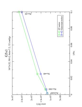
Figure 1: Noise dependence of the $t=1$ element of the $\gamma_{5}\otimes{\bf 1}$ disconnected correlator as a function of the number of noise sources for both $Z_{2}$ and Gaussian noise.

In general one defines noise source vectors $\eta^{i}(x)$ on the entire lattice. The sources obey:

$$\lim_{N_{S}\rightarrow\infty}\frac{1}{N_{S}}\sum_{i=0}^{N_{S}}\eta^{i*}_{x}\eta^{i}_{y}=\delta_{xy},$$ (13)

so that with a large number of sources $N_{S}$ we can solve $\phi_{y}=M^{-1}_{xy}\eta_{y}^{i}$ and then determine the loop operator

$${\mathcal{O}}_{\gamma_{5}\otimes{\bf 1}}(t)= \langle{\rm Tr}\Delta_{xy}M^{-1}_{yx}\rangle$$

$$= \frac{1}{N_{S}}\Bigg{\langle}\sum\limits_{i=0}^{N_{S}}\sum\limits_{{\bf x}}\eta_{x}^{i*}\Delta_{xy}\phi^{i}_{y}\Bigg{\rangle}_{x_{0}=t},$$ (14)

where the operator $\Delta_{xy}$ effects the four-link shift and Kogut-Susskind phasing appropriate for the ${\gamma_{5}\otimes{\bf 1}}$ operator.

3.4 Variance reduction schemes

We have tested a variance reduction trick used by Venkataraman and Kilcup [10]. Specifically, for the $\gamma_{5}\otimes{\bf 1}$ operator we can estimate $\langle{\rm Tr}\Delta_{xy}^{\gamma_{5}\otimes{\bf 1}}M^{-1}_{yx}\rangle$ as

$$\langle{\rm Tr}\Delta_{xy}^{\gamma_{5}\otimes{\bf 1}}M^{-1}_{yx}\rangle=m\Big{\langle}\frac{1}{N_{s}}\sum_{i}\phi_{x}^{i*}\Delta_{xy}^{\gamma_{5}\otimes{\bf 1}}\phi^{i}_{y}\Big{\rangle}.$$ (15)

We note that this expression differs from Eq. 3.3 by $\langle\eta_{x}\mathop{\not\!\!D}(D^{2}+m^{2})^{-1}\eta_{y}\rangle$. The staggered $\mathop{\not\!\!D}$ connects even and odd sites only, and $(M^{\dagger}M)^{-1}=(D^{2}+m^{2})^{-1}$ connects only sites separated by an even number of links. So when $x$ and $y$ are separated by an even number of links this term is zero. This is the case for the four-link $\gamma_{5}\otimes{\bf 1}$, but of course is not for $\gamma_{4}\gamma_{5}\otimes{\bf 1}$. The advantage of this substitution is that while both forms have the same expectation value, the form in Eq. 15 has a smaller variance.

We have also experimented with dilute noise sources. A recent work by the TrinLat Collaboration has suggested that using dilute stochastic sources can reduce the error of quantities measured with stochastic sources [25]. In this scheme the stochastic source vectors are non-zero only on some subset of the lattice, with the set of noise vectors designed such that the entire lattice is covered in the sum over sources. With staggered fermions several different dilution schemes are possible, e.g.: dilution by time-slice, color, site-parity, hypercube component, as well as the intersections of these dilution schemes. We have tested several of dilution schemes and mention the results briefly in subsection 4.2

4 ANALYSIS & RESULTS

4.1 $N_{f}=2+1$ flavor results

Our results to date show a clear signal for connected and disconnected correlators on $N_{f}=0,2$, and $2+1$ lattices. As an example of connected correlators, see Figure 2. The corresponding disconnected correlators are in Figure 3.

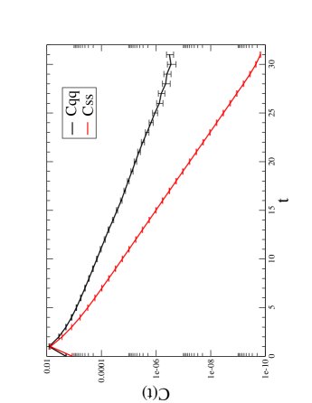
Figure 2: Connected correlators of the $\gamma_{5}\otimes{\bf 1}$ operator for $N_{f}=2+1$ $\beta=6.67$ $am=0.007,0.05$ on $20^{3}\times 64$ lattices.

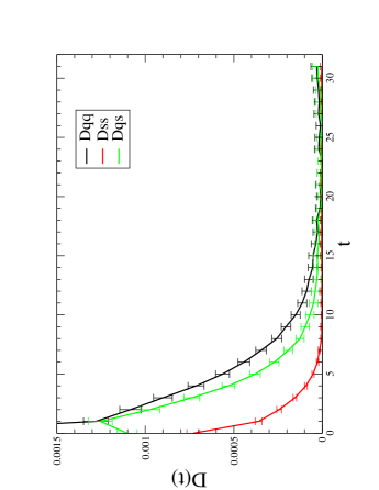
Figure 3: Disconnected correlators of the $\gamma_{5}\otimes{\bf 1}$ operator for $N_{f}=2+1$ $\beta=6.67$ $am=0.007,0.05$ on $20^{3}\times 64$ lattices.

To compute the $D/C$ ratio for the $N_{f}=2+1$ case, we must generalize the definition, (11), of $D/C$. For non-degenerate flavors where the $N_{f}$ total flavors have been separated into $N_{q}$ light flavors and $N_{s}$ strange flavors we must replace:

$$N_{f}^{2}D \longrightarrow N_{q}^{2}D_{qq}+N_{s}^{2}D_{ss}+2N_{q}N_{s}D_{qs}$$ (16)

$$N_{f}C \longrightarrow N_{q}C_{qq}+N_{s}C_{ss}.$$ (17)

Here $D_{qq}$ and $D_{ss}$ are light-light and strange-strange disconnected correlators respectively. $D_{qs}$ is the mixed correlator, with a light quark operator correlated with a strange quark operator. Similarly $C_{qq}$ and $C_{ss}$ are light-light and strange-strange connected correlators respectively. So the $D/C$ ratio generalized for $2+1$ flavors is

$$R(t)=\frac{4D_{qq}+D_{ss}+4D_{qs}}{4C_{qq}+C_{ss}}.$$ (18)

For each ensemble we computed $R(t)$. We show an example of $R(t)$ for $N_{f}=2+1$ flavors in Figure 4. It is here that the limitations of our current statistics begin to show. When we divide the data set into bins of approximately 100 configurations each we note significant differences between the bins in the behavior of $R(t)$ for $t>6$. We attribute this to gauge configuration noise in the disconnected correlator. It suggests that accurate determination of the dynamical staggered pseudoscalar singlet propagator will likely come only with data sets with significantly more configurations. Additional the behavior of $R(t)$ indicates that there may be an inconsistency with the relative normalizations of our connected and disconnected correlators.

4.2 Variance reduction tests

Faced with the the large uncertainties of the disconnected propagator measures in the $N_{f}=2+1$ cases, we tested several several variance reduction schemes to try to improve the signal-to-noise ratio of our disconnected correlators. We ran our disconnected correlator measurement routine on a set of 36 lattices, using a number of different noise vector dilution schemes as well as the Venkataraman-Kilcup variance reduction (VKVR) trick. A comparison is in Figure 5.

There is no doubt that Venkataraman-Kilcup variance reduction is advantageous. In contrast to reference [25], we found no apparent advantages to any of the dilution schemes alone, although it may be possible that with such a small number of lattices, gauge noise overwhelmed the reduction in source noise. There is some suggestion of a slight advantage when time-slice dilution was combined with VKVR. Figure 5 shows a comparison of disconnected correlator error with and without VKVR and time-slice dilution.

It is difficult to make definitive statements without careful error analysis of the variance. The volume filling noise sources can be swapped for time-slice-diluted noise for no extra computational cost and disconnected operators can be computed both with and without VKVR at no extra cost. So both are implemented in our in-progress $N_{f}=2$ and $N_{F}=0$ runs, and will be used in future $N_{f}=2+1$ runs.

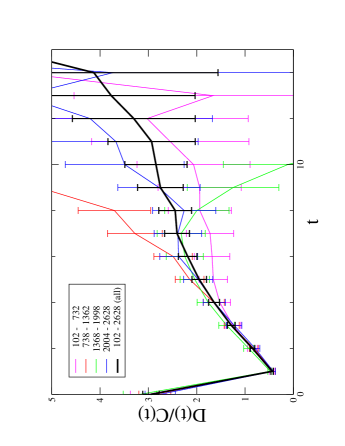
Figure 4: Full $D/C$ ratio for $\gamma_{5}\otimes{\bf 1}$ operator for $N_{f}=2+1$ $\beta=6.67$ $am=0.007,0.05$ on $20^{3}\times 64$ lattices. Bold curve represents data from the full ensemble, while the finer grey curves correspond to bins of one quarter of the ensemble.

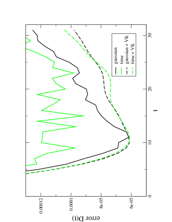
Figure 5: Comparison of disconnected correlator errors using stochastic sources with time-slice dilution and the Venkataraman-Kilcup (VK) trick on 36 $N_{f}=2+1$ $\beta=6.67$ $am=0.01,0.05$ on $20^{3}\times 64$ configurations.

5 CONCLUSIONS & OUTLOOK

We present this as a status report of our staggered pseudoscalar singlet physics project, which is very much a work in progress. We have measured unambiguous signals for connected and disconnected correlators persisting through as many as a dozen time-slices. The gauge error inherent in the disconnected correlators has limited our ability to precisely determine the $D/C$ ratio, and it appears that significantly longer timeseries will be necessary.

In part to meet the significant challenges of measuring disconnected correlators for singlet physics, UKQCD has begun generating the first of several long-timeseries dynamical Asqtad fermion ensembles on the QCDOC machine. Figure 2 lists the lattice sizes and timeseries lengths for the planned ensembles. With these larger ensembles gauge noise should be controlled well enough to make high-precision measurements of the disconnected correlators. At that point it should be possible to not only scrutinize the behavior of the $D/C$ ratio, but variational fitting of the full pseudoscalar singlet propagator should allow determination of both the $\eta$ and $\eta^{\prime}$ meson masses for $N_{f}=2+1$ flavors of dynamical staggered lattice fermions.

$a$ (fm)	$m_{q}/m_{s}$	$L^{3}\times T$	Trajectories
0.125	0.2	$24^{3}\times 64$	30000
0.09	0.2	$32^{3}\times 96$	20000
0.06	0.2	$48^{3}\times 144$	2000

Table 2: Asqtad staggered ensembles planned for generation on the UKQCD’s QCDOC.

References

- [1] E. Witten, Nucl. Phys. B 156 (1979) 269.
- [2] G. Veneziano, Nucl. Phys. B 159 (1979) 213.
- [3] S. Itoh, Y. Iwasaki and T. Yoshie, Phys. Rev. D 36 (1987) 527.
- [4] C. McNeile and C. Michael, Phys. Lett. B 491 (2000) 123, [Erratum-ibid. B 551 (2003) 391].
- [5] T. Struckmann et al., Phys. Rev. D 63 (2001) 074503.
- [6] V. I. Lesk et al., Phys. Rev. D 67 (2003) 074503.
- [7] K. Schilling, H. Neff and T. Lippert, Lect. Notes Phys. 663 (2005) 147.
- [8] C. R. Allton et al., Phys. Rev. D 70 (2004) 014501.
- [9] T. DeGrand and U. M. Heller, Phys. Rev. D 65 (2002) 114501.
- [10] L. Venkataraman and G. Kilcup, [ arXiv:hep-lat/9711006].
- [11] J. B. Kogut, J. F. Lagae and D. K. Sinclair, Phys. Rev. D 58 (1998) 054504.
- [12] C. W. Bernard and M. F. L. Golterman, Phys. Rev. D 46 (1992) 853.
- [13] C. W. Bernard and M. F. L. Golterman, Phys. Rev. D 49 (1994) 486.
- [14] C. W. Bernard et al., Phys. Rev. D 64 (2001) 054506.
- [15] C. Aubin et al., Phys. Rev. D 70 (2004) 094505.
- [16] K. Orginos and D. Toussaint, Phys. Rev. D 59 (1999) 014501.
- [17] K. Orginos, D. Toussaint and R. L. Sugar, Phys. Rev. D 60 (1999) 054503.
- [18] G. P. Lepage, Phys. Rev. D 59 (1999) 074502.
- [19] R. G. Edwards and B. Joo, Nucl. Phys. Proc. Suppl. 140 (2005) 832.
- [20] K. Bitar, et al., Nucl. Phys. B 313 (1989) 348.
- [21] H. R. Fiebig and R. M. Woloshyn, Phys. Rev. D 42 (1990) 3520.
- [22] S. J. Dong and K. F. Liu, Phys. Lett. B 328 (1994) 130.
- [23] Y. Kuramashi, et al., Phys. Rev. Lett. 72 (1994) 3448.
- [24] N. Eicker, et al., Phys. Lett. B 389 (1996) 720.
- [25] J. Foley, et al., arXiv:hep-lat/0505023 (2005).