PQChPT with Staggered Sea and Valence Ginsparg-Wilson Quarks: Vector Meson Masses

Abstract

We consider partially quenched, mixed chiral perturbation theory with staggered sea and Ginsparg-Wilson valence quarks in order to extract a chiral-continuum extrapolation expression for the vector meson mass up to order ${\mathcal{O}}(a^{2})$, at one-loop level. Based on general principles, we accomplish the task without explicitly constructing a sophisticated, heavy vector meson chiral Lagrangian.

year number number identifier

I Introduction

In the past few years there has been significant progress in the study of the chiral-continuum extrapolation problem for lattice QCD with different types of fermions (see, for example, Refs. Bar:2002nr ; Bar:2003mh ; Bar:2005tu ; Tiburzi:2005is ). Extrapolation of lattice QCD simulation results to the physical (light) quark masses is a nontrivial task due to the nonanalytic variation of hadronic properties with quark masses which is a consequence of spontaneous chiral symmetry breaking. To perform an extrapolation to the continuum limit we need to account for direct chiral, taste (in the staggered case) and rotational symmetry breaking by finite lattice spacing.

At present, lattice QCD simulations with staggered fermions defined in Ref. Susskind reached smaller quark masses Bernard:2001av compared with other types of lattice fermions. For example, compared with unquenched simulations using Ginsparg-Wilson fermions (defined in Ref. Ginsparg ) simulations with staggered fermions are computationally less demanding. The computational cost depends on many factors like lattice spacing and the practical implementation of the fermions in the simulations (see Ref. Bar:2005tu and references therein). From Ref. Kennedy:2004ae it follows that the simulations with Ginsparg-Wilson fermions may be about ten to one hundred times more expensive than with improved staggered fermions at comparable masses.

However, the price of these advantages of staggered fermions is that they contain an internal flaw. In those simulations, to reduce the number of taste degrees of freedom, the fourth-root trick is employed. In the continuum limit this trick is consistent because there are no taste-changing interactions, however, when one includes these interactions the finite lattice spacing makes the root of the determinant non-local and the trick remains controversial (see, for example, Ref.Bunk:2004br ). In order to include the relatively large discretization effects in staggered calculations, staggered chiral perturbation theory has been developed (see Refs.Lee:1999zx ; Aubin:2003mg ; Aubin:2003rg ; Sharpe:2004is ). Application of the staggered Lagrangian allowed one to determine the pseudoscalar masses and decay constant Aubin:2003mg ; Aubin:2003rg ; VandeWater:2005uq . For example, recently in Ref. Gray:2005ad there has been considerable success in determining the $B$ meson decay constant using the MILC collaboration unquenched gauge configurations with three flavors of light sea quarks. In these calculations both valence and sea light quarks were represented by the highly improved (AsqTad) staggered quark action which allows for a much smoother chiral extrapolation to physical up and down quarks than has been possible in the past.

Being computationally very costly, Ginsparg-Wilson fermions, on the other hand, do not suffer from the inconsistency of staggered fermions. Moreover, these fermions have an exact chiral symmetry. It has been shown in Refs. Bar:2005tu ; Tiburzi:2005is that it is possible to combine the good chiral properties of Ginsparg-Wilson fermions, taking them as valence quarks where they are computationally less demanding, with numerically fast staggered fermions as sea quarks. Extrapolation for the hybrid (mixed fermion) program has recently been addressed for baryons by Tiburzi in Ref. Tiburzi:2005is . Here we consider the application of this program for the $\rho$ meson, which is a classic testing ground for QCD with light quarks.

In this report we extend the study of QCD for staggered sea and valence Ginsparg-Wilson quarks in Ref.Bar:2005tu to calculate the mass of the vector meson at one-loop level up to order ${\mathcal{O}}(a^{2})$. QCD with staggered sea and valence Ginsparg-Wilson quarks, which as in Bar:2003mh ; Bar:2002nr we will refer to as mixed QCD, consists of $N_{v}$ fully quenched (valence) quarks (with $N_{v}$ ghost-quarks) and $4N_{f}$ staggered (sea) quarks. The masses of the sea and valence quarks, in principle, could be chosen to be completely arbitrary, except that the quenched quark masses are fixed to be equal to the masses of their ghost partners. The full graded chiral symmetry of mixed QCD in the chiral and continuum limits is described via the semi-direct product $G_{MQCD}=SU(4N_{f}+N_{v}|N_{v})_{L}\times SU(4N_{f}+N_{v}|N_{v})_{R}\times U(1)_{V}$, where $4N_{f}$ and $N_{v}$ are the numbers of unquenched (staggered) and quenched quarks, respectively. As in full QCD, we expect that the axial $U(1)_{A}$ symmetry is also broken by the anomaly. We also phenomenologically include in our calculations the one-loop contribution from the $\rho\rightarrow\pi\pi$ decay which cannot be consistently incorporated in the heavy meson formalism because of the high momentum involved in this process. However, the inclusion of this loop is justified by the physical results obtained, for example, in Refs. Allton:2005fb ; Grigoryan:2005zj ; Leinweber:2001ac and references therein.

II Symanzik Action

In order to consistently include lattice discretization effects the Symanzik action Symanzik:1983dc ; Symanzik:1983gh needs to be constructed, based on the symmetry constraints of the underlying lattice theory, with further projection to the low energy effective theory. This task was carried out in Refs.Bar:2005tu ; Tiburzi:2005is and here, we will only briefly mention the main results.

In general, the Symanzik action up to order ${\mathcal{O}}(\epsilon^{4})$ has the form:

$$S_{sym}=S_{PQ}+aS_{1}+a^{2}S_{2}+a^{3}S_{3}+a^{4}S_{4}+\ldots$$ (1)

where $S_{PQ}$ is the action corresponding to continuum partially quenched theory described in Refs. Morel ; Bernard:1993sv , $S_{n}$ ($n\in N$) is the action consisting of dimension $(n+4)$ operators. Here, we will require that the heavy meson chiral Lagrangian, corresponding to $S_{PQ}$, matches the corresponding partially quenched chiral Lagrangian, similar to that in Ref. Chow:1997dw or in Ref. Grigoryan:2005zj when the lattice spacing is set to zero. From discussions in Ref. Tiburzi:2005is (see also Refs. Luscher:1998pq ; Sharpe:1993ng ; Luo:1996vt ) the actions $S_{1}$ and $S_{3}$ are equal to zero because of the specific character of the fermions we use. The action $S_{2}$, according to Ref. Bar:2005tu , contains only six allowed operators which break taste or rotational symmetries (see also for details Refs. Bar:2003mh ; Tiburzi:2005is ; SW ). The chiral Lagrangian corresponding to the action $S_{4}$ will give only a tree level contribution of order ${\mathcal{O}}(a^{4})$. Although allowed in our counting scheme, this contribution will be disregarded, as currently we are interested in the ${\mathcal{O}}(a^{2})$ analytic behavior of vector meson masses.

Using the results from the operator construction in Refs. Bar:2005tu ; Tiburzi:2005is we will study the analytic behavior of the vector meson mass in both the chiral and continuum limits, without constructing the explicit expression for the heavy meson PQChPT.

III Goldstone Meson Multiplet Sector

Mixed ChPT in the Goldstone meson sector with staggered and Ginsparg-Wilson quarks was first studied in Ref.Bar:2005tu . We first give a brief description of that work.

Assuming that the $G_{MQCD}$ symmetry is spontaneously broken down to its vector part, the particle spectrum will contain light pseudoscalar bosons. These Goldstone meson fields can be written in terms of a $(4N_{f}+2N_{v})\times(4N_{f}+2N_{v})$, unitary matrix field, $\Sigma$, defined as:

$$\Sigma=exp(2\imath\Phi/f),$$ (2)

where $\Sigma\in U(4N_{f}+N_{v}|N_{v})$, $\Phi$ is the bosonic matrix and $f$ is a low energy constant. In particular, we are interested in the case with $N_{f}=3$ and $N_{v}=2$, for which the bosonic matrix has the following form:

$$\Phi=\left(\begin{array}[]{ccccccc}U&\pi^{+}&K^{+}&Q_{ux}&Q_{uy}&...&...\\[5.0pt] \pi^{-}&D&K^{0}&Q_{dx}&Q_{dy}&...&...\\[5.0pt] K^{-}&\bar{K}^{0}&S&Q_{sx}&Q_{sy}&...&...\\[5.0pt] Q^{\dagger}_{ux}&Q^{\dagger}_{dx}&Q^{\dagger}_{sx}&X&P^{+}&R^{\dagger}_{\tilde{x}x}&R^{\dagger}_{\tilde{y}x}\\[5.0pt] Q^{\dagger}_{uy}&Q^{\dagger}_{dy}&Q^{\dagger}_{sy}&P^{-}&Y&R^{\dagger}_{\tilde{x}y}&R^{\dagger}_{\tilde{y}y}\\[5.0pt] ...&...&...&R_{\tilde{x}x}&R_{\tilde{x}y}&\tilde{X}&\tilde{P}^{+}\\[5.0pt] ...&...&...&R^{\dagger}_{\tilde{y}x}&R^{\dagger}_{\tilde{y}y}&\tilde{P}^{-}&\tilde{Y}\\[5.0pt] \end{array}\right)$$ (3)

Following the notation of Ref. Bar:2005tu , the following correspondence is implied: $P^{+}\rightarrow x\bar{y}$,   $X\rightarrow x\bar{x}$,   $Y\rightarrow y\bar{y}$,   ($\tilde{P}^{+}$, $\tilde{X}$ and $\tilde{Y}$ are the analogous combinations of valence ghost quarks), $R_{\tilde{x}x}\rightarrow\tilde{x}\bar{x}$, similarly for $R_{\tilde{x}y}$, $R_{\tilde{y}x}$, and $R_{\tilde{y}y}$. $Q_{Fv}\rightarrow F\bar{v}$, where $F\in\{u,d,s\}$ and $v\in\{x,y\}$ (note that $Q_{Fv}$ is a $4\times 1$ matrix in taste). The pseudoscalar states $U$, $D$, $\pi^{+}$,…, etc. in Eq. (3), which consist of staggered quarks only, form the “staggered” sector of the mixed pseudoscalar boson ChPT. This sector is well studied in Refs. Aubin:2003mg ; Aubin:2003rg ; Sharpe:2004is . Each state in the “staggered” sector can be represented as:

$$U=\sum^{16}_{a=1}U_{a}\frac{T_{a}}{2},\ \ \ T_{a}=\{\xi_{5},\imath\xi_{\mu 5},\imath\xi_{\mu\nu},\xi_{\mu},\xi_{I}\}$$ (4)

(similarly for $D$, $K^{+}$, etc ) where $T_{a}$ are the sixteen Euclidean gamma matrices associated with taste (see, for example, Ref.Aubin:2003mg ).

Under chiral symmetry transformations:

$$\Sigma\rightarrow L\Sigma R^{\dagger},$$ (5)

where $L(R)\in SU(4N_{f}+N_{v}|N_{v})_{L(R)}$. As in Refs. Bar:2005tu ; Tiburzi:2005is , we adopt the following counting scheme:

$$m_{q}/\Lambda_{QCD}\approx a^{2}\Lambda^{2}_{QCD}\cong\epsilon^{2},$$ (6)

where $\Lambda_{QCD}$ denotes the typical QCD scale. This counting scheme is relevant for simulations with improved staggered quarks Aubin:2004fs . The leading order chiral Lagrangian (in this counting scheme) that contains the terms of order ${\mathcal{O}}(p^{2},m_{q},a^{2})$ is of the form:

$$L_{\Phi}=\frac{f^{2}}{8}<\partial_{\mu}\Sigma\partial^{\mu}\Sigma^{\dagger}>-\ \frac{f^{2}B}{4}<\Sigma M^{\dagger}+\ \Sigma^{\dagger}M>+\ \frac{m^{2}_{0}}{6}<\Phi^{2}>+\ a^{2}{\mathcal{V}}.$$ (7)

Here $<...>$ denotes a supertrace in flavor space and $B$ is a low-energy constant. In our case the diagonal mass matrix is:

$$M=diag(m_{u}\xi_{I},m_{d}\xi_{I},m_{s}\xi_{I},m_{x},m_{y},m_{x},m_{y}).$$ (8)

For convenience, to derive the flavor neutral propagators, the singlet mass parameter $m^{2}_{0}$ in Eq. (7) is allowed to be finite, however, at the end of the calculations we always could take the limit $m^{2}_{0}\rightarrow\infty$.

The potential ${\mathcal{V}}$ in the leading order Lagrangian comprises all terms proportional to $a^{2}$. At this stage we will not go deep into describing the form of the ${\mathcal{V}}$ (we refer to Refs. Bar:2005tu ; Aubin:2003mg for more information). Here, we present only those results required for our further study.

At tree level, because of the specific properties of potential ${\mathcal{V}}$, the valence-valence mesons with only Ginsparg-Wilson quarks obey the continuum-like mass relations:

$$m^{2}_{P}=B(m_{x}+m_{y}),\ \ \ \ m^{2}_{X(Y)}=2Bm_{x(y)}.$$ (9)

In our calculations the only relevant valence-valence Goldstone bosons will be flavor neutral because the valence quarks in the sea loops will be canceled by their ghost partners and, in addition, G-parity suppresses the process $\rho\rightarrow\eta^{\prime}\pi$. We also will be interested only in flavor-neutral and taste singlet staggered quark combinations, so in the sea-sea sector, for a meson in a singlet taste channel $I$ made of sea quarks of flavor $F$, we have:

$$m^{2}_{F_{I}}=2Bm_{F}+a^{2}\Delta_{I}$$ (10)

where the constant $\Delta_{I}$ is given, for example, in Ref. Bar:2005tu (Eq. (27)). Finally, the masses of the valence-sea mesons ($F\bar{v}$ or $\bar{F}v$) are given as:

$$m^{2}_{Q_{Fx(y)}}=B(m_{F}+m_{x(y)})+a^{2}\Delta_{Mix},$$ (11)

where $\Delta_{Mix}$ is an undetermined parameter in this mixed theory which is taste independent.

The flavor-charged (non-diagonal) fields in Eq. (3) have only connected propagators ($G^{con}_{ij}$), in the quark-flow sense, which are given by the expression:

$$G^{con}_{ij}(p)=\frac{\delta_{ij}\epsilon_{i}}{p^{2}+m^{2}_{ii}}$$ (12)

where $i$, $j$ $\in$ {ghost, quark}, $\epsilon_{i}=1$ if $i=$ quark and $-1$ if $i=$ ghost. Disconnected propagators for flavor neutral mesons (like, for example, $U$ or $X$) contain hairpin-like interactions (through the $m^{2}_{0}$ term). The sum of all these hairpin-like diagrams (in the way described in Ref.Aubin:2003mg ) for the disconnected $XY$ propagators ($G^{disc}[XY]$) will give (as in Ref. Bar:2005tu ) the following result:

$$G^{disc}[XY]=-\frac{m^{2}_{0}}{3}\frac{(q^{2}+m^{2}_{U_{I}})(q^{2}+m^{2}_{D_{I}})(q^{2}+m^{2}_{S_{I}})}{(q^{2}+m^{2}_{X})(q^{2}+m^{2}_{Y})(q^{2}+m^{2}_{\pi^{0}_{I}})(q^{2}+m^{2}_{\eta_{I}})(q^{2}+m^{2}_{\eta^{\prime}_{I}})}$$ (13)

where $\pi^{0}_{I}$ , $\eta_{I}$ and $\eta^{\prime}_{I}$ are the diagonalized flavor-neutral, singlet taste-channel mass eigenstates. Although there should be vector and axial-vector hairpin contributions, as in Ref. Aubin:2003mg , we do not include them here because they are irrelevant in our later calculations.

IV Mixed One-Loop Corrections to the Vector Meson Mass

ChPT with staggered sea and chiral (Ginsparg-Wilson) valence quarks was successfully applied to calculate the corrections to pseudoscalar masses and decay constants to one loop in Ref. Bar:2005tu and recently, in Ref. Tiburzi:2005is , this approach was applied to calculate masses and magnetic moments of baryons. In this work we will calculate vector meson mass corrections at one-loop level, without explicitly constructing the corresponding heavy meson Lagrangian but rather using general principles.

From Eq. (1) it follows that continuum heavy meson chiral Lagrangian will consist of the parts: $L_{1}\sim{\mathcal{O}}(p)\sim{\mathcal{O}}(\epsilon)$ and $L_{2}\sim{\mathcal{O}}(m_{q})\sim{\mathcal{O}}(\epsilon^{2})$. As shown in Ref. Grigoryan:2005zj , from the comparison with the simulations in Ref. Allton:2005fb , the contribution from the terms of order ${\mathcal{O}}(m^{2}_{q})$ may be neglected. The chiral Lagrangian, $L_{b}$, corresponding to $S_{2}$ in Eq. (1), will consist of terms of order ${\mathcal{O}}(a^{2})\sim{\mathcal{O}}(\epsilon^{2})$. And finally, we will not have terms of order ${\mathcal{O}}(p^{n+1})$ ($n\in N$) in the heavy meson chiral Lagrangian because they can be eliminated by using the equations of motion Arzt:1993gz .

Now, it is easy to see that $L_{1}$ gives one-loop chiral corrections to the vector meson mass – see the diagrams $(a,c,d)$ shown in Fig. 1. The terms in $L_{2}$ and $L_{b}$ will give tadpole as well as tree level contributions. From these considerations for the total tree level correction $\sigma_{tree}$ to the vector meson mass (up to order ${\mathcal{O}}(\epsilon^{4})$) it follows that:

$$\sigma_{tree}(\mu)=c_{1}a^{2}+c_{2}m_{x}+c_{3}m_{y}+c_{4}m_{u}+c_{5}m_{d}+c_{6}m_{s}$$ (14)

where, in general, $c_{i}=c_{i}(\mu)$ ($i=1,...,6$) with $\mu$ as the renormalization scale.

For concreteness we will calculate the mass correction of a charged $\rho$ meson at rest. (The calculation is somewhat more complicated for a neutral $\rho$ meson, but because of isospin symmetry, the mass correction of all $\rho$ mesons must be the same.)

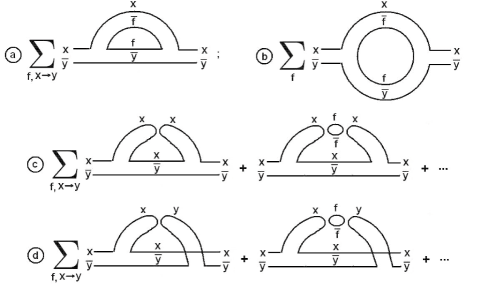
Figure 1: The quark flow diagrams

In the case $N_{f}=3$ and $N_{v}=2$ we have staggered $u$, $d$ and $s$ sea quarks with $x$ and $y$ valence quenched quarks (corresponding to different flavors). The quark flow diagrams for this case are presented in Fig. 1, with the propagators for the connected diagrams (Fig. 1 $a,b$) given by:

$$G^{con}_{vvp} =\sum_{f=u,d,s}\left[\frac{1}{(q^{2}+m^{2}_{Q_{fx}})}+\frac{1}{(q^{2}+m^{2}_{Q_{fy}})}\right]\frac{1}{((p-q)^{2}+M^{2})}\ ,$$

$$G^{con}_{vpp} =\sum_{f=u,d,s}\frac{1}{(q^{2}+m^{2}_{Q_{fx}})((p-q)^{2}+m^{2}_{Q_{fy}})},$$ (15)

where $p$ is the initial momentum of the vector meson with mass $M$ ($p^{2}=-M^{2}$ in Euclidean space), $q$ is the momentum of intermediate pseudoscalar meson state and instead of using a heavy meson propagator we just used the usual one (which is practically the same) with the mass of intermediate vector meson equal to the mass of the initial one. The subindices on the propagators remind us that in the self-energy integral we need to take into account the vector-vector-pseudoscalar ($vvp$) and vector-pseudoscalar-pseudoscalar ($vpp$) nature of the meson interactions. For the diagrams in Fig. 1$c$ and $d$ in the limit $m_{0}\rightarrow\infty$, we have:

$$G^{DHP}_{vvp}=-\frac{1}{3}\frac{(q^{2}+m^{2}_{U_{I}})(q^{2}+m^{2}_{D_{I}})(q^{2}+m^{2}_{S_{I}})}{(q^{2}+m^{2}_{\pi^{0}_{I}})(q^{2}+m^{2}_{\eta_{I}})((p-q)^{2}+M^{2})}\left[\frac{1}{(q^{2}+m^{2}_{X})}+\frac{1}{(q^{2}+m^{2}_{Y})}\right]^{2}.$$ (16)

Notice, that for case shown in Fig. 1$b$ there are no additional double hairpin diagrams because of G-parity. Now, let us take $m_{u}=m_{d}\equiv m$ ($N_{f}=2+1$ picture) as in MILC simulations Aubin:2004wf . In this case:

$$m^{2}_{U_{I}}=m^{2}_{D_{I}}=m^{2}_{\pi^{0}_{I}}$$

$$m^{2}_{\eta_{I}}=\frac{1}{3}m^{2}_{U_{I}}+\frac{2}{3}m^{2}_{S_{I}}$$ (17)

Let us also require that $m_{x}=m_{y}$ and $m_{U_{I}}=m_{X}$ or equivalently $Bm_{x}=Bm+\frac{1}{2}a^{2}\Delta_{I}$. The first choice will help us to find the correction to the $\rho$ meson mass because it consists of two light quarks. The second choice is natural because in the continuum limit it gives $m_{x}=m$. Taking these two conditions into account we can write the above propagator in the form:

$$G^{DHP}_{vvp}=-\frac{2}{3}\left[\frac{3}{q^{2}+m^{2}_{X}}-\frac{1}{q^{2}+m^{2}_{\eta_{I}}}\right]\frac{1}{((p-q)^{2}+M^{2})}.$$ (18)

Using the method in Ref. Pichowsky:1999mu for the total self-energy we have:

$$\Sigma_{total} =\sum_{f=u,d,s}\left(2\Sigma_{vvp}(M^{2},m^{2}_{Q_{fx}},\Lambda)+\Sigma_{vpp}(m^{2}_{Q_{fx}},\Lambda)\right)$$ (19)

$$-2\Sigma_{vvp}(M^{2},m^{2}_{X},\Lambda)+\frac{2}{3}\Sigma_{vvp}(M^{2},m^{2}_{\eta_{I}},\Lambda)$$

where

$$\Sigma_{vvp}(M^{2},m^{2},\Lambda) =-\frac{g^{2}M}{12\pi^{2}}\int^{\infty}_{0}dk\frac{k^{4}u^{2}_{vvp}(k^{2},\Lambda)}{\omega^{2}},$$ (20)

$$\Sigma_{vpp}(m^{2},\Lambda) =-\frac{f^{2}_{\rho\pi\pi}}{6\pi^{2}}\int^{\infty}_{0}dk\frac{k^{4}u^{2}_{vpp}(k^{2},\Lambda)}{\omega(\omega^{2}-\frac{M^{2}}{4})},$$ (21)

we used the notation $\omega^{2}=k^{2}+m^{2}$ and the functions $u^{2}_{vvp(vpp)}(k^{2},\Lambda)$ are finite range regulators (Pichowsky:1999mu ; Leinweber:2001ac ; Donoghue:1998bs ; Detmold:2001hq ). For example, the leading non-analytic (LNA) contribution to the self energy is:

$$\Sigma^{LNA}_{total} =-\frac{g^{2}M}{24\pi}\left(4m^{3}_{Q_{ux}}+2m^{3}_{Q_{sx}}-2m^{3}_{X}+\frac{2}{3}m^{3}_{\eta_{I}}\right)$$ (22)

In the continuum limit (where we have $m_{x}=m$) the LNA contribution is:

$$\delta M^{LNA} =\frac{\Sigma^{LNA}_{total}}{2M}=-\frac{g^{2}}{48\pi}\left(2m^{3}_{\pi}+2m^{3}_{K}+\frac{2}{3}m^{3}_{\eta}\right).$$ (23)

This result agrees with that in Ref. Jenkins:1995vb for the vector $\rho$ meson - where in the limit $N_{c}\rightarrow\infty$ they found:

$$\delta M^{LNA}_{\rho}=-\frac{g^{2}_{2}}{12\pi f^{2}}\left[2m^{3}_{\pi}+2m^{3}_{K}+\frac{2}{3}m^{3}_{\eta}\right].$$ (24)

Note that while the coefficients in these two expressions are written differently, since $g=2g_{2}/f$ for values of $g\equiv g_{\rho\omega\pi}=16$ $GeV^{-1}$ (Leinweber:2001ac ), $g_{2}=0.75$ (Jenkins:1995vb ) and $f=93.75$ $MeV$, the expressions are equal.

It would be also interesting to consider the case, when $m_{u}=m_{d}$, $m_{X}=m_{U_{I}}$ and $m_{Y}=m_{S_{I}}$ ($m_{y}=m_{s}$ in the continuum limit). Using these conditions and recalling that the $K^{*}$ vector meson consists of one light and one strange quark we find the self energy contribution:

$$\Sigma_{total}=\sum_{f=u,d,s}\left(\Sigma_{vvp}(M^{2},m^{2}_{Q_{fx}},\Lambda)+\Sigma_{vvp}(M^{2},m^{2}_{Q_{fy}},\Lambda)+\Sigma_{vpp}(m^{2}_{Q_{fx}},m^{2}_{Q_{fy}},\Lambda)\right)-$$ (25)

$$-\frac{1}{2}\Sigma_{vvp}(M^{2},m^{2}_{X},\Lambda)-\Sigma_{vvp}(M^{2},m^{2}_{Y},\Lambda)+\frac{1}{6}\Sigma_{vvp}(M^{2},m^{2}_{\eta_{I}},\Lambda)$$

In the continuum limit ($m_{x}=m_{u}$ and $m_{y}=m_{s}$) the LNA contribution to the total self-energy is:

$$\Sigma^{LNA}_{total}=\frac{g^{2}_{2}}{12\pi f^{2}}\left(\frac{3}{2}m^{3}_{\pi}+3m^{3}_{K}+\frac{1}{6}m^{3}_{\eta}\right).$$ (26)

Again, comparing this result with that in Ref. Jenkins:1995vb for the $K^{*}$ meson mass correction (in the limit $N_{c}\rightarrow\infty$):

$$\delta M_{K^{*}}=-\frac{g^{2}_{2}}{12\pi f^{2}}\left[\frac{3}{2}m^{3}_{\pi}+3m^{3}_{K}+\frac{1}{6}m^{3}_{\eta}\right]$$ (27)

we see good agreement with our result for the LNA contribution in the continuum limit.

Now, returning to $\rho$ meson, let us take into account the tadpole contribution from $L_{2(b)}\sim{\mathcal{O}}(a^{2},m_{q})$. This case is similar to $L_{1}$ but without intermediate vector meson propagators and we don’t need to include the diagram with two intermediate pseudoscalars. The total self-energy correction from $L_{2(b)}$ is:

$$\widetilde{\Sigma}_{total}=4\Sigma_{tad}(m^{2}_{Q_{ux}},\Lambda)+2\Sigma_{tad}(m^{2}_{Q_{sx}},\Lambda)-2\Sigma_{tad}(m^{2}_{X},\Lambda)+\frac{2}{3}\Sigma_{tad}(m^{2}_{\eta_{I}},\Lambda),$$ (28)

with the definition:

$$\Sigma_{tad}(m^{2},\Lambda)=\tilde{\beta}\int\frac{d^{4}k}{(2\pi)^{4}}\frac{k^{2}u^{2}(k^{2},\Lambda)}{(k_{0}-\imath\epsilon)^{2}(k^{2}+m^{2}+\imath\epsilon)},$$ (29)

where, in general, $\tilde{\beta}=\beta^{\prime}m^{2}+\beta a^{2}$, $\beta^{\prime}$ and $\beta$ are undetermined parameters and $u(k^{2},\Lambda)$ is a finite range regulator Leinweber:2001ac ; Donoghue:1998bs ; Detmold:2001hq . The term proportional to $\beta^{\prime}$ is absent in the continuum limit (see, for example, Ref. Grigoryan:2005zj when lattice spacing is set to zero). This means that the tadpole contribution comes only from the operators in $L_{b}$. Then, for example, if $u=1$ (applying dimensional regularization) we have:

$$\Sigma_{tad}(m^{2})=\frac{\beta a^{2}}{16\pi^{2}}m^{2}ln\frac{m^{2}}{\mu^{2}}\sim{\mathcal{O}}(\epsilon^{4}).$$ (30)

The calculations above were performed in the case where $x$ and $y$ correspond to different flavors. To calculate the mass of the neutral vector meson we need to change our quark flow diagrams and add one more with DHP insertions on each intermediate pseudoscalar line. However, as noted above, isospin symmetry for the vector meson, means that we need not perform separate calculations for the neutral vector meson mass.

V Vector Meson Masses up to order ${\mathcal{O}}(\epsilon^{4})$

Imposing the conditions $m_{x}=m_{y}=m_{u}+\frac{1}{2B}a^{2}\Delta_{I}$ with $m_{u}=m_{d}$ we can simplify the expression for the tree level contribution and the vector meson mass in both chiral and continuum expansions can be written in the form:

$$M^{2}_{V}=\left(c+c_{a}a^{2}+c_{q}m^{2}_{\pi}+c_{s}m^{2}_{S_{I}}\right)^{2}+\Sigma_{total}(\mu)+\widetilde{\Sigma}_{total}(\mu),$$ (31)

where $m^{2}_{\pi}=2Bm_{x}=m^{2}_{X}$, $m^{2}_{S_{I}}=2Bm_{s}+a^{2}\Delta_{I}$ and $c$, $c_{a,q,s}$ are new dimensionful parameters. The dependence on $m^{2}_{S_{I}}$ may be absorbed in the coefficients $c$ and $c_{a}$ if one fixes the mass of the strange quark in the simulations.

From the definition of $\Sigma_{vvp}$ and $\Sigma_{vpp}$ using the appendix in Ref. Leinweber:2001ac we can separate the leading non-analytic contributions from $\Sigma_{total}$ and $\widetilde{\Sigma}_{total}$

$$\Sigma^{LNA}_{total} =-\frac{\mu_{\rho}g^{2}}{12\pi}\left(2m^{3}_{Q_{ux}}+m^{3}_{Q_{sx}}-m^{3}_{X}+\frac{1}{3}m^{3}_{\eta_{I}}\right)$$

$$\ \ \ \ \ \ \ \ \ \ \ \ \ \ -\frac{f^{2}_{\rho\pi\pi}}{4\pi^{2}\mu^{2}_{\rho}}\left[2m^{4}_{Q_{ux}}ln\frac{m_{Q_{ux}}}{\mu}+m^{4}_{Q_{sx}}ln\frac{m_{Q_{sx}}}{\mu}\right],$$ (32)

$$\widetilde{\Sigma}^{LNA}_{total} =\frac{\beta a^{2}}{8\pi^{2}}\left[2m^{2}_{Q_{ux}}ln\frac{m_{Q_{ux}}}{\mu}+m^{2}_{Q_{sx}}ln\frac{m_{Q_{sx}}}{\mu}-m^{2}_{X}ln\frac{m_{X}}{\mu}+\frac{1}{3}m^{2}_{\eta_{I}}ln\frac{m_{\eta_{I}}}{\mu}\right]$$

where $\mu_{\rho}$ is the physical mass of the $\rho$ meson and using Eqs. (9–11) we can express all meson masses as functions of $m^{2}_{\pi}$ and $m^{2}_{S_{I}}$:

$$m^{2}_{Q_{ux}} =m^{2}_{\pi}+a^{2}\left(\Delta_{Mix}+\frac{1}{2}\Delta_{I}\right),$$ (33)

$$m^{2}_{Q_{sx}} =\frac{1}{2}m^{2}_{\pi}+\frac{1}{2}m^{2}_{S_{I}}+a^{2}\left(\Delta_{Mix}-\frac{1}{2}\Delta_{I}\right),$$ (34)

$$m^{2}_{\eta_{I}} =\frac{1}{3}m^{2}_{\pi}+\frac{2}{3}m^{2}_{S_{I}}.$$ (35)

It is also of practical interest to consider the general case with only two conditions: $m_{u}=m_{d}$ and $m_{x}=m_{y}$. In this case the total self-energies are:

$$\Sigma_{total} =\sum_{f=u,d,s}\left(2\Sigma_{vvp}(M^{2},m^{2}_{Q_{fx}},\Lambda)+\Sigma_{vpp}(m^{2}_{Q_{fx}},\Lambda)\right)$$

$$-\frac{4}{3}\alpha\Sigma_{vvp}(M^{2},m^{2}_{X},\Lambda)-\frac{4}{3}(1-\alpha)\Sigma_{vvp}(M^{2},m^{2}_{\eta_{I}},\Lambda)+\frac{4}{3}\tilde{\alpha}\frac{\partial\Sigma_{vvp}(M^{2},m^{2}_{X},\Lambda)}{\partial m^{2}},$$

$$\widetilde{\Sigma}_{total} =4\Sigma_{tad}(m^{2}_{Q_{ux}},\Lambda)+2\Sigma_{tad}(m^{2}_{Q_{sx}},\Lambda)$$

$$-\frac{4}{3}\alpha\Sigma_{tad}(m^{2}_{X},\Lambda)-\frac{4}{3}(1-\alpha)\Sigma_{tad}(m^{2}_{\eta_{I}},\Lambda)+\frac{4}{3}\tilde{\alpha}\frac{\partial\Sigma_{tad}(m^{2}_{X},\Lambda)}{\partial m^{2}},$$

where

$$\alpha =1-\frac{m^{2}_{\eta_{I}}-m^{2}_{S_{I}}}{m^{2}_{\eta_{I}}-m^{2}_{X}}+\frac{(m^{2}_{\eta_{I}}-m^{2}_{S_{I}})(m^{2}_{U_{I}}-m^{2}_{X})}{(m^{2}_{\eta_{I}}-m^{2}_{X})^{2}}$$

$$\tilde{\alpha} =(m^{2}_{U_{I}}-m^{2}_{X})\left[1-\frac{m^{2}_{\eta_{I}}-m^{2}_{S_{I}}}{m^{2}_{\eta_{I}}-m^{2}_{X}}\right]$$

from which one can see if $m_{X}=m_{\pi}=m_{U_{I}}$ then we have the same result as in Eqs. (25,28).

To perform chiral-continuum extrapolation of lattice data for the $\rho$ meson with Ginsparg-Wilson quarks in a staggered sea the consistent numerical evaluation of self-energy integrals $\Sigma_{total}(\mu)$ and $\tilde{\Sigma}_{total}(\mu)$ needs to be done using the particular type of finite range regulator. The extrapolation formula, in a numerical simulation with fixed strange quark mass, will have five coefficients, some of which are functions of the FRR cutoff.

VI Conclusion

Based on the recently developed mixed PQChPT for pseudoscalar meson sector we have extracted a chiral-continuum extrapolation formula for the vector meson masses at one-loop up to order ${\mathcal{O}}(a^{2})$. Instead of writing explicit expression for the vector meson Lagrangian we have used general principles in order to calculate the mass corrections at one-loop order.

Up to order ${\mathcal{O}}(\epsilon^{4})$, vector meson masses, in general, depend on six, presently unknown, parameters: $c$, $c_{a,q,s}$, $\beta$ and $\Delta_{Mix}$. The low energy coefficient $\Delta_{Mix}$ is model independent and may also be estimated from the extrapolation of pseudoscalar masses. If one, however, is interested in vector meson mass corrections up to order ${\mathcal{O}}(\epsilon^{3})$ then the number of parameters reduces by two:

$$M^{2}_{V}=\left(c+c_{a}a^{2}+c_{q}m^{2}_{\pi}+c_{s}m^{2}_{S_{I}}\right)^{2}-\frac{\mu_{\rho}g^{2}}{12\pi}\left(2m^{3}_{Q_{ux}}+m^{3}_{Q_{sx}}-m^{3}_{X}+\frac{1}{3}m^{3}_{\eta_{I}}\right).$$ (36)

This can be used to test the theory predictions up to order ${\mathcal{O}}(\epsilon^{3})$. It is also possible to reduce the number of extrapolation parameters by one if we fix the strange quark mass in the simulations.

During the derivations the following approximations were used: $m_{x}=m_{y}$, $m_{u}=m_{d}$ and $m_{X}=m_{U_{I}}$ for the $\rho$ meson. This approximation may be adjusted, for example, to the $K^{*}$ vector meson if we assume $m_{u}=m_{d}$, $m_{X}=m_{U_{I}}$ and $m_{Y}=m_{S_{I}}$. The idea beyond this is that in the continuum limit the masses of the valence quarks, $m_{x}$ and $m_{y}$, are required to correspond to the masses of valence quarks from which the vector meson is constructed.

In our calculations we include (phenomenologically) the relativistic $\rho\rightarrow\pi\pi$ decay process, which although cannot be consistently included in the framework of low energy effective field theory, is required to give consistent physical predictions. Finally, we did not take into account the finite volume effects from the lattice, which are already well studied in Refs. Arndt:2004bg ; Bedaque:2004dt ; Orth:2005kq ; Colangelo:2004sc .

References

- (1) O. Bär et al., Phys. Rev. D 67, 114505 (2003) [arXiv:hep-lat/0210050].
- (2) O. Bär et al., Phys. Rev. D 70, 034508 (2004) [arXiv:hep-lat/0306021].
- (3) O. Bär et al., Phys. Rev. D 72, 054502 (2005) [arXiv:hep-lat/0503009].
- (4) B. C. Tiburzi, arXiv:hep-lat/0508019.
- (5) L. Susskind, Phys. Rev. D 16, 3031 (1977).
- (6) C. W. Bernard et al., Phys. Rev. D 64, 054506 (2001) [arXiv:hep-lat/0104002].
- (7) P. H. Ginsparg and K. G. Wilson, Phys. Rev. D 25, 2649 (1982).
- (8) A. D. Kennedy, Nucl. Phys. Proc. Suppl. 140, 190 (2005) [arXiv:hep-lat/0409167].
- (9) B. Bunk et al., Nucl. Phys. B 697, 343 (2004) [arXiv:hep-lat/0403022].
- (10) W. J. Lee and S. R. Sharpe, Phys. Rev. D 60, 114503 (1999) [arXiv:hep-lat/9905023].
- (11) R. S. Van de Water and S. R. Sharpe, arXiv:hep-lat/0507012.
- (12) C. R. Allton et al., Phys. Lett. B 628, 125 (2005) [arXiv:hep-lat/0504022].
- (13) C. Aubin and C. Bernard, Phys. Rev. D 68, 034014 (2003) [arXiv:hep-lat/0304014].
- (14) C. Aubin and C. Bernard, Nucl. Phys. Proc. Suppl. 129, 182 (2004) [arXiv:hep-lat/0308036].
- (15) S. R. Sharpe and R. S. Van de Water, Phys. Rev. D 71, 114505 (2005) [arXiv:hep-lat/0409018].
- (16) A. Gray et al. [HPQCD Collaboration], arXiv:hep-lat/0507015.
- (17) H. R. Grigoryan and A. W. Thomas, arXiv:hep-lat/0507028, to appear in Phys. Lett. B.
- (18) D. B. Leinweber et al., Phys. Rev. D 64, 094502 (2001) [arXiv:hep-lat/0104013].
- (19) K. Symanzik, Nucl. Phys. B 226, 187 (1983).
- (20) K. Symanzik, Nucl. Phys. B 226, 205 (1983).
- (21) A. Morel, J. Phys. (France) 48, 1111 (1987).
- (22) C. W. Bernard and M. F. L. Golterman, Phys. Rev. D 49, 486 (1994) [arXiv:hep-lat/9306005].
- (23) C. K. Chow and S. J. Rey, Nucl. Phys. B 528, 303 (1998) [arXiv:hep-ph/9708432].
- (24) M. Luscher, Phys. Lett. B 428, 342 (1998) [arXiv:hep-lat/9802011].
- (25) B. Sheikholeslami and R. Wohlert, Nucl. Phys. B 259, 572 (1985).
- (26) S. R. Sharpe, Nucl. Phys. Proc. Suppl. 34, 403 (1994) [arXiv:hep-lat/9312009].
- (27) C. Aubin et al. (MILC), Phys. Rev. D 70, 114501 (2004) [arXiv:hep-lat/0407028].
- (28) Y. b. Luo, Phys. Rev. D 55, 353 (1997) [arXiv:hep-lat/9604025].
- (29) C. Arzt, Phys. Lett. B 342, 189 (1995) [arXiv:hep-ph/9304230].
- (30) C. Aubin et al., Phys. Rev. D 70, 094505 (2004) [arXiv:hep-lat/0402030].
- (31) M. A. Pichowsky et al., Phys. Rev. D 60, 054030 (1999) [arXiv:nucl-th/9904079].
- (32) J. F. Donoghue et al., Phys. Rev. D 59, 036002 (1999) [arXiv:hep-ph/9804281].
- (33) W. Detmold et al. Pramana 57, 251 (2001) [arXiv:nucl-th/0104043].
- (34) E. Jenkins et al., Phys. Rev. Lett. 75, 2272 (1995) [arXiv:hep-ph/9506356].
- (35) D. Arndt and C. J. D. Lin, Phys. Rev. D 70, 014503 (2004) [arXiv:hep-lat/0403012].
- (36) P. F. Bedaque et al. Phys. Rev. D 71, 054015 (2005) [arXiv:hep-lat/0407009].
- (37) B. Orth et al. Phys. Rev. D 72, 014503 (2005) [arXiv:hep-lat/0503016].
- (38) G. Colangelo, Nucl. Phys. Proc. Suppl. 140, 120 (2005) [arXiv:hep-lat/0409111].