We explore gauge actions for lattice QCD, which are constructed such that the occurrence of small plaquette values is strongly suppressed. By choosing strong bare gauge couplings we arrive at values for the physical lattice spacings of ${\cal O}(0.1~{}{\rm fm})$. Such gauge actions tend to confine the Monte Carlo history to a single topological sector. This topological stability facilitates the collection of a large set of configurations in a specific sector, which is profitable for numerical studies in the $\epsilon$-regime. The suppression of small plaquette values is also expected to be favourable for simulations with dynamical quarks. We use a local Hybrid Monte Carlo algorithm to simulate such actions, and we present numerical results for the static potential, the physical scale, the topological stability and the kernel condition number of the overlap Dirac operator. In addition we discuss the question of reflection positivity for a class of such gauge actions.

1 Introduction

The gauge action of QCD can be lattice discretised in many ways. One requires the naive continuum limit for all lattice gauge actions to coincide, and one usually assumes that then they fall into the same universality class. The formulation of the lattice gauge actions is considered less problematic than the fermionic part of QCD, in particular due to the absence of additive mass renormalisation. Even for the simplest plaquette action, known as the Wilson gauge action [1],

$$S_{\rm W}[U]=\beta\sum_{P}S_{P}(U_{P})\ ,\quad S_{P}(U_{P})=1-\frac{1}{3}{\rm Re~{}Tr}U_{P}\ ,$$ (1.1)

the lattice artifacts in the scaling behaviour only appear in ${\cal O}(a^{2})$, where $a$ is the lattice spacing. This is in contrast to the Wilson fermion, which suffers from ${\cal O}(a)$ artifacts, as well as additive mass renormalisation, so that criticality can only be approached with a tedious fine tuning.

Nevertheless there are a number of suggestions for improved lattice gauge actions. In general the goal is to further suppress the scaling artifacts by including more extended closed loops in the discrete formulation of the field strength tensor. This is achieved for instance by the tree level improved Symanzik gauge action [3], the on-shell improved Lüscher-Weisz action [4], and by several renormalisation group improved actions [5, 6, 7].

In the current work we also consider non-standard gauge actions for lattice QCD, but we focus on another property, which we want to improve. Our intention is to suppress as far as possible the occurrence of small plaquette values. Of course, this suppression prevents the gauge field from fluctuating as it would for the Wilson gauge action, hence we have to use much stronger bare gauge couplings to arrive at a comparable lattice spacing. For practical simulations a lattice spacing of ${\cal O}(0.1~{}{\rm fm})$ is required; this enables the use of a sensible physical volume with lattices of a tractable size. For quenched simulations with the Wilson gauge action such a lattice spacing is obtained for $\beta=6/g_{0}^{2}\approx 6$. We will see that a lattice spacing of the same magnitude can still be obtained for the actions that drastically suppress small plaquette values, if we drive $\beta$ down to values around and even below 1.

This observation means that these gauge actions can in fact be used in simulations. Now we would like to explain what virtues we expect from it.

2 Motivations for the suppression of small plaquette values

Small plaquette values $U_{P}$ are expected to be linked to small eigenvalues of the Dirac operator, which is most relevant in view of dynamical simulations. On the practical side, the suppression of small values for $U_{P}$ should speed up dynamical Hybrid Monte Carlo (HMC) simulations, avoid problems with the numerical integrator and ease the access to light pions. This would mean a further improvement in this direction, in addition to recent algorithmic developments [8]. However, these properties are not tested in the current work; we leave them for further investigation.

We do investigate, however, another virtue, which we want to explain now. There is a notorious lack of analytical tools to handle QCD at low energy, so one often switches to the use of an effective Lagrangian instead. In particular, chiral perturbation theory ($\chi$PT) is an effective theory in terms of the Nambu-Goldstone boson fields of chiral symmetry breaking [9]. This approach is very powerful, and it still works if one includes the small explicit chiral symmetry breaking due to the finite masses of the light quarks. Then one deals with light pseudo Nambu-Goldstone bosons, which are identified with the light mesons. However, by its nature $\chi$PT cannot capture all the properties of QCD as the fundamental theory. To supplement the missing information, in particular the values of the Low Energy Constants in the chiral Lagrangian, one has to relate $\chi$PT to QCD results, which one tries to obtain from lattice simulations, so we need simulations with light mesons.

In the recent years, a lattice fermion formulation became available, which overcomes the conceptual problems related to the chiral symmetry. This is the case if a lattice Dirac operator $D$ obeys the Ginsparg-Wilson (GW) relation [10, 11]. In its simplest form (and in lattice units, $a=1$) the GW relation reads

$$D\gamma_{5}+\gamma_{5}D=\frac{1}{\mu}D\gamma_{5}D\ ,\qquad\mu\mathop{\raise 1.29167pt\hbox{$>$\kern-7.5pt\raise-4.73611pt\hbox{$\sim$}}}1\ .$$ (2.1)

The corresponding GW fermions have a lattice modified, but exact chiral symmetry at arbitrary lattice spacing, with the full number of generators [12]. This property rules out additive mass renormalisation (along with ${\cal O}(a)$ scaling artifacts). Hence a small (bare) quark mass $m_{q}$ does indeed imply a small pion mass, $m_{\pi}^{2}\propto m_{q}$.

In practice, there are still difficulties left when we want to approach the physical pion mass. To illuminate this point, we look at the Neuberger overlap operator [13], which is an often applied, explicit solution to the GW relation. At zero fermion mass it takes the form

$$D_{\rm ov}^{(0)}=\mu\Big{[}1+\gamma_{5}Q/\sqrt{Q^{2}}\Big{]}\ ,\quad Q=\gamma_{5}(D_{\rm W}-\mu)\ ,$$ (2.2)

where $D_{\rm W}$ is the Wilson Dirac operator. Its property $D_{\rm W}^{\dagger}=\gamma_{5}D_{\rm W}\gamma_{5}$ implies that $Q$ is Hermitian. A quark mass is added to the overlap operator as follows,

$$D_{\rm ov}(m_{q})=\Big{(}1-\frac{m_{q}}{2\mu}\Big{)}D_{\rm ov}^{(0)}+m_{q}\ .$$ (2.3)

Simulations with this operator are computationally expensive, so that the corresponding QCD studies are essentially restricted to the quenched approximation up to now. The trouble-maker is the inverse square root, which has to be approximated by polynomials of a high degree. The effort to handle $D_{\rm ov}$ is roughly proportional to this degree, which grows — for a fixed accuracy of $D_{\rm ov}$ — like the square root of the condition number of $Q^{2}$. (One usually projects out the lowest few modes and treats them separately to lower this condition number, but this takes time again.) The lowest eigenvalues of $Q^{2}$ are again expected to be linked to the occurrence of low plaquette values. We are going to demonstrate an improvement also in this respect for the gauge actions that we are going to consider.

Another obvious problem at small pion mass are the finite size effects. In a box of side length $L$ they depend on the product $m_{\pi}L$, which should be large to keep the finite size effects small, i.e. to be close to the physically realistic situation. Then we are in the $p$-regime, where the $p$-expansion of $\chi$PT [14] applies. For instance, for $a=0.1~{}{\rm fm}$ a pion mass of $250~{}{\rm MeV}$ corresponds to a correlation length $\xi=1/m_{\pi}$ of about 8 lattice spacings, and to dwarf the finite size effects $L$ should be much larger. Lattices of such an extent are very expensive with GW fermions, even quenched, still without reaching physical pion masses.

As a way out one may consider the opposite situation,

$$\xi\leq L\ ,$$ (2.4)

where we are confronted with strong finite size effects. This setting is called the $\epsilon$-regime; it allows for the use of a variant of chiral perturbation theory known as the $\epsilon$-expansion [15]. It describes the finite size effects analytically, and its formulae can be related to the numerically measured finite size effects. The interesting point is that these formulae involve the Low Energy Constants as they appear in infinite volume. Therefore we can extract physically relevant information even from the unphysical $\epsilon$-regime.

As a peculiarity of the $\epsilon$-regime, the topology plays an important rôle. Observables tend to depend significantly on the topological sector, and predictions exist for expectation values in specific sectors [16]. Therefore, for numerical measurements it can be advantageous, if not necessary, to disentangle the topologies, in order to extract maximal information.

In general, it is not obvious how to define topological sectors on the lattice, since all gauge configurations can be continuously deformed into one another. A neat definition exists, however, for Ginsparg-Wilson fermions, since they have exact zero modes with definite chiralities [11]. Once a GW operator is chosen, it has for each gauge configuration a well-defined fermion index

$$\nu=n_{+}-n_{-}\ ,$$ (2.5)

where $n_{\pm}$ is the number of zero modes with positive/negative chirality. In the spirit of the Atiyah-Singer Theorem one then uses this index as a definition of the topological charge. For independent configurations the distribution of $\nu$ is Gaussian, and its width determines the topological susceptibility.

Let us assume that we monitor the deformation of a gauge configuration to a different topological charge $\nu$ — defined by the overlap operator given in eq. (2.2). In the (real) spectrum of the operator $Q$ such a change of $\nu$ means that some eigenvalue crosses zero (on the topological boundary the overlap operator is not defined). For a transition the Monte Carlo history has to pass through a region of rather low probability, and in simulations one assumes this to happen quickly at some instances in a long history. For simulations in the $p$-regime one tries to sample all topologies and frequent transitions are therefore desired. However, in $\epsilon$-regime simulations one would often like to collect statistics at one specific value of $|\nu|$ to measure an expectation value in this sector. For the parameters that have been used in the $\epsilon$-regime simulations [17, 18, 19, 20, 21, 22, 23, 24, 25], it would be of particular interest to collect large sets of configurations with $|\nu|=1$ and $2$. The topologically neutral sector is problematic due to the frequent appearance of very small Dirac eigenvalues, which leads to strong spikes in the Monte Carlo histories of correlation functions [20] (at $|\nu|>0$ the non-zero eigenvalues are pushed to higher energies [26, 18]). However, a procedure called Low Mode Averaging was designed to render also the neutral sector tractable [22], hence also a cumulation of configurations with $\nu=0$ may be of interest (see also Ref. [24]). Charged sectors are required, however, for the method of extracting Low Energy Constants solely from the zero mode correlation functions [21, 23].

A box with $V\approx 10~{}{\rm fm}^{4}$ is suitable, but the width of the Gaussian charge distribution is then around $\langle\nu^{2}\rangle\approx 10$ [19, 23], so that most charges vary between about $-10$ and $10$. The index measurement by itself is computationally expensive, hence identifying a set of, say, ${\cal O}(1000)$ configurations in one sector is a tedious task — if one uses the standard Wilson gauge action.

Therefore it is motivated to modify the lattice gauge action such that topological transitions are suppressed. The vicinity of a transition (under a continuous deformation) is characterised again by the occurrence of small plaquette values, hence the technical aim is also in that respect to avoid these configurations. This connection was made rigorous first in Ref. [28]. If we consider the overlap operator (2.2), the square root cannot vanish — and therefore topological transitions are excluded under continuous deformations — if all the plaquette variables $U_{P}$ in the configurations involved obey the inequality (at $\mu=1$)

$$S_{P}(U_{P})<\varepsilon=\frac{2}{5d(d-1)}=\frac{1}{30}\ ,$$ (2.6)

where $S_{P}$ represents the standard gauge action of one plaquette, as specified in eq. (1.1). Then the topological structure is continuum-like.

Later on H. Neuberger showed that this constraint can be relaxed a little by increasing the threshold in inequality (2.6) to [29]

$$\varepsilon=\frac{1}{(1+1/\sqrt{2})d(d-1)}\simeq\frac{1}{20.5}\ .$$ (2.7)

This constraint ensures that the spectrum of $Q^{2}$ (the argument of the square root in the overlap formula (2.2)) is strictly positive. In absence of zero modes this condition also guarantees the locality of the overlap operator (in the sense of an exponential decay) [28].

On the other hand, the impact of imposing such a restrictive constraint strictly could be a severe practical problem. The fluctuations of the gauge field would be limited so much that one could only obtain a tiny physical lattice spacing, and therefore a tiny physical volume. However, even for simulations in the $\epsilon$-regime we have to require that the spatial box length $L$ exceeds some lower limit in the range of $L\mathop{\raise 1.29167pt\hbox{$>$\kern-7.5pt\raise-4.73611pt\hbox{$\sim$}}}1.1~{}{\rm fm}\dots 1.5~{}{\rm fm}$ (depending on the exact criterion) [18, 19, 20, 21, 22, 23, 24].

Here we present numerical experiments with gauge actions which do suppress small plaquette values, but only to the extent that still allows for a reasonable physical lattice spacing to be obtained. Then there is no rigorous guarantee for topology conservation in the Monte Carlo history. The hope is that the transitions are still strongly suppressed, so that the history has periods of constant charge, which are sufficiently long to allow us to collect many configurations in a specific sector. Moreover, if we can be confident that topological transitions rarely happen, most of the index computation can be omitted; one would just check after a number of configurations if the index has not changed.

Of course, these configurations should sample independently the observables to be measured in a fixed topology. Since we aim at long sequences of fixed topological charge, this can also be interpreted as a long topological autocorrelation time. Of course, at the same time, we aim at a much shorter autocorrelation time for other observables. We repeat that a long topological autocorrelation is something one would not wish in general — for instance simulations in the $p$-regime — but in the $\epsilon$-regime this property turns into an advantage, if the observables of interest are still weakly autocorrelated.

3 The gauge actions

We now describe a number of non-standard lattice gauge actions, which suppress the undesired small plaquette values. As long as the action for very smooth configurations — with $S_{P}\mathop{\raise 1.29167pt\hbox{$>$\kern-7.5pt\raise-4.73611pt\hbox{$\sim$}}}0$ for all plaquettes — is not altered, the naive continuum limit coincides with the one of the Wilson action (1.1), and with continuum QCD. The suppression becomes strong when $S_{P}$ reaches the value of some parameter $\varepsilon$, which one would theoretically choose according to eq. (2.7). For practical purposes we will have to relax $\varepsilon$ to larger values. A simple cutoff for $S_{P}$ at this value would be conceivable, but such a discontinuity in the action (which would then suddenly jump to infinity) does not appear promising. We can still impose a cutoff but let the plaquette action diverge continuously as $S_{P}$ increases towards $\varepsilon$, if we modify $S_{P}$ of eq. (1.1) to the hyperbolic form

$$S_{\varepsilon,n}^{\rm hyp}(U_{P})=\left\{\begin{array}[]{cc}\frac{S_{P}(U_{P})}{[1-S_{P}(U_{P})/\varepsilon]^{n}}&{\rm~{}~{}for~{}~{}}S_{P}(U_{P})<\varepsilon\\ +\infty&{\rm otherwise}\end{array}\right.$$ (3.1)

for $n>0$. This formulation, with $n=1$, was introduced by M. Lüscher and used for conceptual studies of chiral gauge theories on the lattice [31]. In that case, $\varepsilon$ was of course set to a theoretically stringent value.

In simulations, this action was first used in the Schwinger model by H. Fukaya and T. Onogi [32]. They set $\varepsilon=1$, i.e. far above the theoretical value of about $0.29$, but they still observed topological stability over hundreds of trajectories.

A theoretical objection against this lattice action was raised by M. Creutz [33]. He observed that it does not provide a positive definite transfer matrix. Of course, if we rely on the assumption that we are in the same universality class as the Wilson action (as the naive continuum limit suggests) then one would not worry about that, since the non-positivity would be a cut-off effect and we expect positivity to be restored in the continuum limit. Still, a problem with this action cannot be strictly excluded. Therefore we kept this point in mind in the numerical study and we will comment on it in Subsection 4.3.

The infinite part in action (3.1) means that certain steps that the HMC algorithm suggests have to be rejected for sure. Therefore we also have to verify with special care that the acceptance rate is sufficiently high.

This motivated us to consider further variants of gauge actions, which also suppress the probability of plaquette actions $S_{P}>\varepsilon$, but which do not render a violation of this constraint completely impossible. Examples for such actions are the “power actions”and the “exponential actions”,

$$S_{\varepsilon,n}^{\rm pow}(U_{P}) = S_{P}(U_{P})+\frac{1}{\varepsilon}S_{P}(U_{P})^{n}\ ,$$ (3.2)

$$S_{\varepsilon,n}^{\rm exp}(U_{P}) = S_{P}(U_{P})\cdot\exp\{S_{P}(U_{P})^{n}/\varepsilon\}\qquad(n>0)\ .$$ (3.3)

In our numerical studies we included the actions $S_{\varepsilon,1}^{\rm hyp}$ and $S_{\varepsilon,8}^{\rm exp}$. Our preliminary results were reported in Refs. [34] and a comprehensive presentation will be given in the next Section. Further results along these lines for quenched QCD can be found in Refs. [35, 36].

4 Numerical results

Actions of the types (3.1), (3.2) and (3.3) depend non-linearly on the link variables $U_{x,\mu}$. As a consequence, the heat-bath algorithm and over-relaxation cannot be applied straightforwardly. Therefore we use the local HMC algorithm, which was introduced in Ref. [37]. Since these actions are still composed of separate contributions by the single plaquettes, the force in the local HMC algorithm is a simple modification of the corresponding force for the Wilson action,

$$F^{\rm hyp}_{\varepsilon,n}=\frac{\delta S^{\rm hyp}_{\varepsilon,n}(U_{P})}{\delta U_{x,\mu}}=F^{\rm W}(U_{P})\cdot\frac{1+\frac{n-1}{\varepsilon}S_{P}(U_{P})}{[1-\frac{1}{\varepsilon}S_{P}(U_{P})]^{n+1}}$$ (4.1)

$$F^{\rm exp}_{\varepsilon,n}=\frac{\delta S^{\rm exp}_{\varepsilon,n}(U_{P})}{\delta U_{x,\mu}}=F^{\rm W}(U_{P})\cdot\Big{(}1+\frac{n}{\varepsilon}S_{P}(U_{P})^{n-1}\Big{)}\,\exp\Big{\{}\frac{1}{\varepsilon}S_{P}(U_{P})^{n}\Big{\}}$$ (4.2)

$${\rm where}\qquad F^{\rm W}(U_{P})=\frac{\delta S_{P}(U_{P})}{\delta U_{x,\mu}}$$

is the force of the Wilson action, and its modification by the second factor is of order ${\cal O}(S_{P}/\varepsilon)$ in both cases. This is illustrated in Figure 1.

Figure 1: On the left: The ratio between the hyperbolic plaquette action (for $n=1$) and standard plaquette action, and the corresponding ratio for the exponential actions with $n=1$ and $n=8$ (the latter is that case we studied). On the right: the same ratios for the HMC forces, again as a function of $S_{P}$.

In such simulations, it is also of special importance to check that the results do not depend on the starting configuration (once we start in the desired topological sector). It would be conceivable that the constraint on the plaquette values causes also unwanted obstructions. For all the quantities to be considered below, it turned out that this was not the case; an example is discussed in Subsection 4.6.

4.1 Plaquette values

As a first experiment we considered action (3.1) and searched for the lines of a constant mean plaquette action $\langle S_{P}\rangle$ on a $4^{4}$ lattice, as $\beta$ and the action parameter $\varepsilon$ are varied. The result is shown in Figure 2. As we decrease $\varepsilon$, very small values of $\beta$, i.e. strong bare gauge couplings are needed to keep $\langle S_{P}\rangle$ constant.

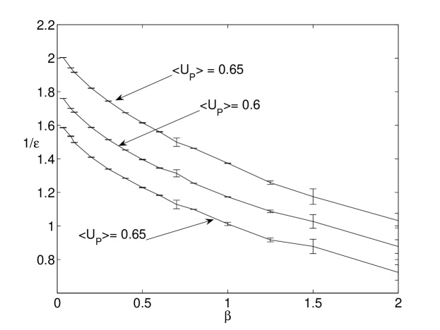
Figure 2: The lines of constant plaquette values in the plane spanned by $1/\varepsilon$ and $\beta$, on a $4^{4}$ lattice.

Next we took a look at the statistical distribution of the plaquette actions, and we show corresponding histograms in Figure 3. By decreasing the values of $\varepsilon$ and $\beta$ we can in fact keep $\langle S_{P}\rangle$ approximately constant, while drastically suppressing the occurrence of very small plaquette actions.

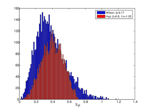
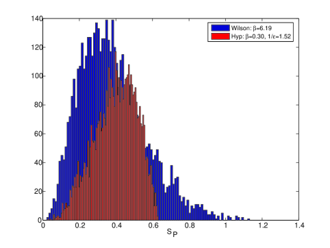
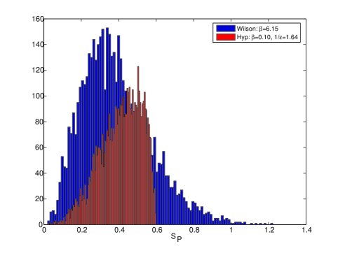
Figure 3: Examples for the histograms of plaquette actions $S_{P}(U_{P})$ with hyperbolic topology conserving actions $S_{\varepsilon,1}^{\rm hyp}$ at various parameters, compared to the Wilson action, on a $4^{4}$ lattice.

However, for a systematic approach to identify a line of a constant physical scale, we have to proceed to larger lattices and we determine the physical scale based on the static potential, since the plaquette value cannot be used for this purpose. This issue will be discussed in the next Subsection.

4.2 The static potential and the physical scale

A very well established method for setting a scale in pure gauge theory is based on the measurement of the static potential at intermediate distances. This potential, and the resulting force, are extracted from the Wilson loop correlations at sufficiently large time separations, such that excited states can be neglected.

To suppress the effects of short-ranged fluctuations, we applied APE smearing [38] on the spatial links before evaluating the Wilson loops. Then we evaluated the static potential

$$aV(r)=\ln\left(\frac{W(r,t-a)}{W(r,t)}\right)\ ,$$ (4.3)

where $W(r,t)$ is a rectangular Wilson loop with extension $r$ and $t$ in a spatial and in the temporal direction (and $V(r)$ is extracted from an asymptotic window in $t$). Here we applied the variational procedure explained in Refs. [39, 40]. The force $F(r)$ is then obtained from the discrete gradient of $V(r)$. The aim is to fix the quantity $r_{0}=0.5~{}{\rm fm}$ [41] by tuning the dimensionless term

$$r^{2}F(r)|_{r=r(c)}=c\ ,\quad r_{0}=r(1.65)\ .$$ (4.4)

To this end, we applied a local interpolation for the force based on the ansatz

$$F(r)=f_{1}+f_{2}r^{2}\ .$$ (4.5)

The results for the action $S^{\rm hyp}_{\varepsilon,1}$ at different values of $\varepsilon$ and $\beta$ are shown in Table 1. From the scale $r_{0}/a$ we can identify an “equivalent” $\beta$-value for the Wilson gauge action, which we denote by $\beta_{\rm W}$. It corresponds to the same lattice spacing for the plaquette action (1.1), where we refer to the parametrisation formula in Ref. [39].

$1/\varepsilon$	$\beta$	$r_{0}/a$	$\beta_{W}$	$d\tau$	$\tau^{\rm plaq}$	$f_{\rm top}$	$\tau^{\rm plaq}\cdot f_{\rm top}$	acc. rate
0.	6.18	7.14(3)	6.18	0.1	7(1)	2.2(13) e-2	$\approx$ 1.5 e-1	$>$ 99 %
1.	1.5	6.6(2)	6.13(2)	0.1	2.2(1)	3.0(23) e-3	$\approx$ 6.6 e-3	$>$ 99 %
1.	1.5	6.6(2)	6.13(2)	0.05	2.0(1)	2.9(11) e-3	$\approx$ 5.8 e-3	$>$ 99 %
1.	1.5	6.6(2)	6.13(2)	0.01	2.2(1)	3.5(8) e-3	$\approx$ 7.7 e-3	$>$ 99 %
1.	1.5	6.6(2)	6.13(2)	0.005	2.3(2)	2.8(15) e-3	$\approx$ 6.4 e-3	$>$ 99 %
1.18	1.	7.2(2)	6.18(2)	0.1	1.2(1)	2.0(12) e-3	$\approx$ 2.4 e-3	$>$ 99 %
1.18	1.	7.2(2)	6.18(2)	0.02/0.01	1.3(1)	1.6(7) e-3	$\approx$ 2.1 e-3	$>$ 99 %
1.25	0.8	7.0(1)	6.17(1)	0.1	1.1(1)	2.3(13) e-3	$\approx$ 2.5 e-3	$>$ 99 %
1.52	0.3	7.3(4)	6.19(4)	0.1	0.8(1)	9.0(28) e-4	$\approx$ 7.2 e-4	$\approx$ 95 %
1.64	0.1	6.8(3)	6.15(3)	0.1	1.0(1)	1.3(7) e-3	$\approx$ 1.3 e-3	$\approx$ 65 %
1.64	0.1			0.05	0.7(1)	2.3(13) e-3	$\approx$ 1.6 e-3	$\approx$ 78 %
1.64	0.1			0.025	0.6(1)	3.5(20) e-3	$\approx$ 2.1 e-3	$\approx$ 93 %
1.64	0.1			0.001	0.5(1)	3.7(23) e-3	$\approx$ 1.9 e-3	$\approx$ 99 %

Table 1: Results for the hyperbolic actions $S^{\rm hyp}_{\varepsilon,1}$, defined in eq. (3.1), for different values of $\varepsilon$ and $\beta$, on a $16^{4}$ lattice. We first show the ratio $r_{0}/a$, which fixes the physical scale. For comparison we also display the $\beta$-values $\beta_{\rm W}$, which leads to the same physical scale for the Wilson action (1.1) [39]. The trajectories were all of length 1 and divided into HMC steps of length $d\tau$. For the plaquette values this leads to a mean autocorrelation time $\tau^{\rm plaq}$, which we show as an example for the autocorrelation of a non-topological quantity. The topological stability, on the other hand, is measured by the frequency of topological transitions. More precisely, $f_{\rm top}$ is the number of topological jumps (determined from cooling), normalised by the number of trajectories. Its product with $\tau^{\rm plaq}$ characterises the dominance of the topological autocorrelation. Finally we give the acceptance rate of the local HMC algorithm. For each set of parameters in this Table we collected at least 200 thermalised configurations spaced by 50 trajectories each. A detailed discussion is given in the following Subsections.

$1/\varepsilon$	$\beta$	$r_{0}/a$	$\beta_{W}$	$d\tau$	$\tau^{\rm plaq}$	$f_{\rm top}$	$\tau^{\rm plaq}\cdot f_{\rm top}$	acc. rate
500	0.044	$>8.5$	$>6.30$	0.015	0.6(1)	2.5(36) e-4	$\approx$ 1.5 e-4	$\approx$ 99%
600	0.0134	8.0(2)	6.26(1)	0.015	0.6(1)	2.5(23) e-4	$\approx$ 1.5 e-4	$\approx$ 99%
1000	0.004	$>9$	$>6.34$	0.03	0.6(1)	0(0)		$\approx$ 25%
1000	0.00113	7.9(1)	6.25(1)	0.015	0.6(1)	1.7(23) e-4	$\approx$ 1.0 e-4	$\approx$ 99%

Table 2: Results for the exponential actions $S^{\rm exp}_{\varepsilon,8}$, defined in eq. (3.3), for different values of $\varepsilon$ and $\beta$, on a $16^{4}$ lattice. As in Table 1 we first show the ratio $r_{0}/a$ and the Wilson $\beta$-value $\beta_{\rm W}$, which leads to the same physical scale for the Wilson action (1.1) (here the finite size effects in the evaluation of $r_{0}/a$ may be sizable). For different HMC steps $d\tau$ we then give the mean plaquette autocorrelation time $\tau^{\rm plaq}$, the frequency of topological transitions, $f_{\rm top}$, its product with $\tau^{\rm plaq}$ and the acceptance rate. The number of measurements for $r_{0}/a$ was at least 200 in each case. Further comments are added in Subsections 4.4 and 4.6.

Let us comment now on the possible errors in this evaluation:

• The systematic error on the interpolation can be estimated by considering a third point and observe the relative deviation between the two interpolations; in our case this error turned out to be negligible compared to the statistical uncertainties.

• Previous computations [39] revealed that for a box size $L\gtrsim 3.3\;r_{0}$ the finite size effects for the computation of $r_{0}$ can be safely neglected. The same work observed that for the Wilson action at $\beta=5.95$ and $L\simeq 2.4\,r_{0}$ the finite size artifacts of the force amount to $\approx\;3\%$. In our study we deal with $L=16\simeq(2.2\dots 2.4)\;r_{0}$. Hence we assume finite size effects for $r_{0}$ to be of this order as well.

• The errors quoted on $r_{0}/a$ in Table 1 and 2 are purely statistical (they were computed by the jackknife method). The same errors are shown in Figures 4 and 5, which we comment on below. The extent of these errors is acceptable in this context, since a precise determination of $r_{0}$ was not the purpose of this work, so we did not aim at high statistics.

• A way to check the lattice artifacts is to compare the short distance force at finite lattice spacing with the one extrapolated to the continuum limit in Ref. [40]. In particular we measured the ratio

  $$\Delta(r/r_{0})=\frac{r^{2}F(r/r_{0})-r^{2}F(r/r_{0})|_{c}}{r^{2}F(r/r_{0})|_{c}}\ ,$$ (4.6)

  where $r^{2}F(r/r_{0})|_{c}$ denotes the continuum limit. The results for the action $S^{\rm hyp}_{\varepsilon,1}$ are shown in Figure 4. At short distances, lattice artifacts are below $15\%$ for all the different values of $1/\varepsilon$ and $\beta$ that we included. Moreover, one observes that discretisation errors grow substantially for increasing values of $1/\varepsilon$, as expected. This indicates that choosing even larger values of $1/\varepsilon$ — while keeping the physical lattice spacing fixed — could introduce sizeable cutoff effects.

  

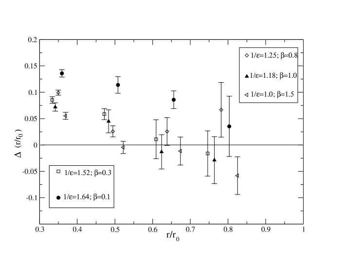
  Figure 4: Lattice artifacts for the action $S^{\rm hyp}_{\varepsilon,1}$. The plot shows the relative deviation of the force $r^{2}F(r)$ from the continuum results, given in eq. (4.6).

• For the Wilson action it turned out that the lattice artifacts can be reduced considerably by using a so-called “tree level improved” definition of the force. For this purpose, one defines an improved distance $r_{I}$ such that the force does not contain lattice artifacts at tree level,

  $$F(r_{I})=\frac{4}{3}\frac{g_{0}^{2}}{4\pi r_{I}^{2}}+\mathcal{O}(g_{0}^{4})\ .$$ (4.7)

  If we adapt this method, the procedure described before leads to the results shown in Figure 5. For the largest values of $1/\varepsilon$ one observes some reduction of the lattice artifacts, whereas they seem to increase for the smallest $1/\varepsilon$. This behaviour is not totally surprising, since it has been observed in other cases that this improvement is not always guaranteed [42].
  We also observe that the use of tree-level improved observables does not change the results for $r_{0}/a$ itself (within the statistical errors).

• For a comparison of the scaling quality one may, for instance, refer to the Iwasaki action [5] (at $r_{0}/a\simeq 6.0$) and the DBW2 action [6] (at $r_{0}/a\simeq 5.5$) at a distance $r/r_{0}\approx 0.3$: in these cases the lattice artifacts were found to be of order $\sim 10\%$ [42]. Those discretisation errors are therefore comparable to our results for the actions $S^{\rm hyp}_{\varepsilon,1}$.

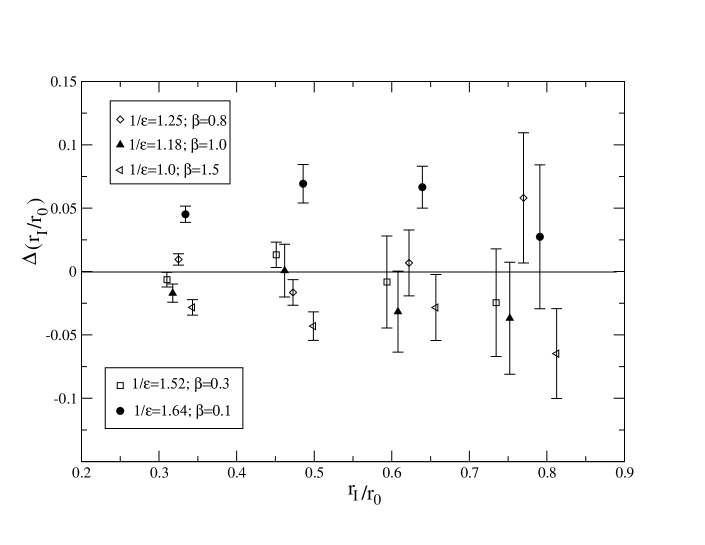
Figure 5: Lattice artifacts for the action $S^{\rm hyp}_{\varepsilon,1}$ with a tree level improved definition of the force (4.7). The plot shows the relative deviation of the force $r^{2}F(r)$ from the continuum results.

We repeat that our statistics is modest, and our intention in this analysis was only to check whether the errors and lattice artifacts are reasonably under control. This can be confirmed from the results shown Figures 4 and 5, and the accuracy is fully sufficient for our purposes.

4.3 The issue of reflection positivity

As we anticipated in Section 3, Ref. [33] pointed out that actions of the type (3.1) do not provide a positive transfer matrix, as it was observed [43] a long time ago for the so-called Manton action [44]. The positivity of the transfer matrix is assured if positivity holds for both, “site reflection” and “link reflection” (e.g. reflections on the hyperplanes $x_{4}=0$ and $x_{4}=1/2$).

However, this still leaves the possibility of obtaining a positive squared transfer matrix. In fact, this is the case if the action obeys at least one of the two reflection positivities [2]. We have checked for the actions involved in our study, given in eqs. (3.1) and (3.3), that site reflection positivity does in fact hold.

From the practical point of view, the lack of positivity can be reflected in an irregular behaviour of the effective potential $V(r,t)$ at short time separation, as observed in Ref. [41] for actions involving rectangular loops (like those suggested in Refs. [4, 5, 6]). This is a lattice artifact which does, in principle, not constitute a problem, as long as one keeps far enough from the cutoff. In the case of the actions considered in this work and with our statistical precision, such an irregular behaviour could not been observed in the extraction of the static potential.

4.4 Acceptance rate

Also the problem related to the acceptance rate has been mentioned in Section 3. This point motivated us to consider also a set of exponential actions of the type (3.3), in addition to the hyperbolic actions, and the corresponding results are given in Table 2. In both cases, the acceptance rate is very high for most of the actions we studied. It drops, however, if one pushes for very low values of $\varepsilon$ (along with an extremely small $\beta$). As the last lines in Table 1 show, the acceptance rate can actually be driven up again even at $1/\varepsilon=1.64$ by using very short HMC steps. However, this cannot be considered a solution, because it increases the costs (especially in the dynamical case), and also the frequency of topological transitions rises again (c.f. Subsection 4.6).

Therefore, this property sets another limit on the suppression of the small plaquette values, in addition to the scaling of the static potential at short distances.

4.5 The condition number for the overlap operator

This Subsection discusses the condition number of the operator $Q^{2}$, which is crucial for the computational effort required to deal with the overlap operator in eq. (2.2). Table 3 collects our results for the action $S^{\rm hyp}_{1,\varepsilon}$ compared to $S_{\rm W}$, at the values of $\varepsilon$ and $\beta$ corresponding to approximately constant physics according to Table 1. Similar results were presented in Refs. [36], which also include first tests with dynamical overlap fermions.

In our study we varied the parameter $\mu$ by units of $0.1$ and found the optimal condition numbers for all gauge actions involved at $\mu=1.6$. For the case of 10 eigenmodes of $Q^{2}$ projected out, this property can be seen in the upper plot of Figure 6. Hence we compare the condition numbers at $\mu=1.6$ for different gauge actions in Table 3 and in the lower plot of Figure 6. These results are based on 30 configurations in each case.

$\beta$	$1/\varepsilon$	$c_{2}$	$c_{6}$	$c_{11}$	$c_{21}$
6.17	0	1051(369)	575(110)	461(46)	390(30)
6.18	0	723(294)	501(43)	424(27)	371(16)
6.19	0	872(499)	506(57)	437(25)	374(16)
1.5	1	453(101)	360(30)	325(11)	294(7)
1	1.18	390(34)	328(18)	302(10)	281(9)
0.8	1.25	439(89)	341(23)	311(15)	285(9)
0.3	1.52	369(41)	301(13)	280(7)	263(5)
0.1	1.64	433(82)	342(18)	315(14)	293(8)

Table 3: Condition numbers $c_{n}$ of the operator $Q^{2}$ in the square root of the Neuberger overlap operator at $\mu=1.6$, after projecting out the leading $n-1$ modes of $Q^{2}$. In this comparison we always considered configurations generated by the local HMC algorithm with $d\tau=0.1$.

Figure 6: Comparison of the condition number $c_{11}$ for various values of $\mu$ (on top), and $c_{n}$ for running $n$ at $\mu=1.6$ (below), for different types of gauge actions. (The parameters $\mu$ and $c_{n}$ are defined in eqs. (2.2) and (4.8).)

We show the condition numbers

$$c_{n}:=\lambda_{\rm max}/\lambda_{n}\ ,\quad(\lambda_{\rm max},\ \lambda_{n}\ :\ {\rm largest~{}resp.~{}n^{th}~{}eigenvalue~{}of~{}}Q^{2})$$ (4.8)

which are relevant after projecting out the leading $n-1$ modes of $Q^{2}$. We see that the $c_{n}$ are indeed lowered as $1/\varepsilon$ increases, which reduces the effort for overlap fermion simulations. If $n$ is around 20, then — for the smooth configurations that we considered here — the gain compared to $S_{\rm W}$ is only moderate. However, for the hyperbolic actions $S^{\rm hyp}_{1,\varepsilon}$ the number of these modes can be reduced drastically without much loss in the condition number of the remaining operator. This is in contrast to $S_{\rm W}$, and it matters in applications, since the special treatment of each of these projected modes also takes computation time (although this is typically a minor part of the total computational effort).

4.6 Topological charge stability

For a quick analysis, we used the cooling method [46] to estimate the topological charge. The resulting topological stability over the trajectories is included in Tables 1 and 2. In independent tests we evaluated for a subset of the configurations the overlap indices setting $\mu=1.3$, $1.4$, $1.5$, $1.6$ and $1.7$. Since we are dealing with smooth configurations, it does not come as a surprise that we found an excellent agreement of more than 98 % for all these definitions of the topological charge, i.e. the charges obtained with cooling and the overlap index at any of the parameters $\mu$ listed up above. Hence the results in the Tables are relevant for the overlap index as well.

As a more direct illustration, we show typical histories of the topological charge (defined by cooling) for different parameters in Figure 7.

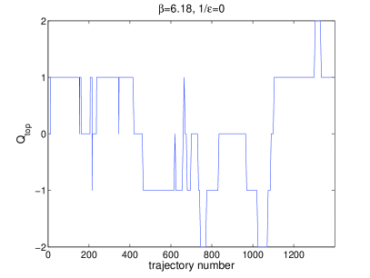
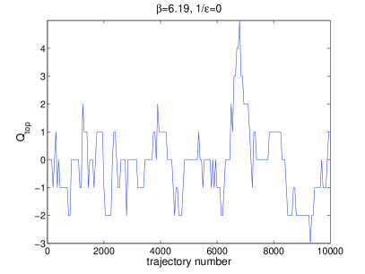
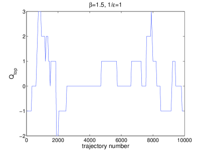
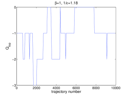
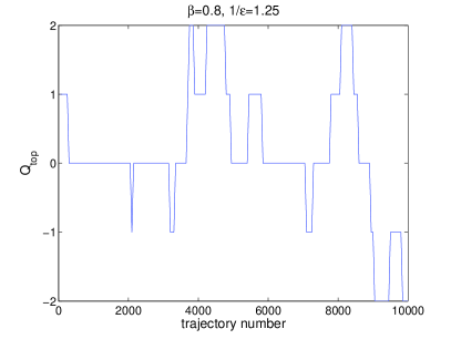
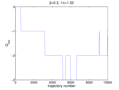
Figure 7: Typical histories of the topological charge for the actions $S_{\rm W}$ (on top) and $S_{\varepsilon,1}^{\rm hyp}$ at various combinations of $\varepsilon$ and $\beta$, as in Table 1. We show results obtained on a $16^{4}$ lattice with the HMC step size $d\tau=0.1$. We see that an increased $1/\varepsilon$ keeps the charge more and more stable.
The charge was measured by cooling once in 50 trajectories, except for the plot at $\beta=6.18$, where measurements were made every single or every 5 trajectories. Notice, on the other hand, that in the plot at $\beta=6.19$ the assumption that the separation of measurements is much larger than the typical distance of topology changes is not justified, and the frequency of topological transitions based on this plot would be underestimated.

To measure the stability of the topological sector, we monitored the number of charge changes normalised by the number of trajectories. We denote this parameter as the “frequency of topological transitions”, $f_{\rm top}$, and give results in Tables 1 and 2.

As we already mentioned in Subsection 4.4, for a fixed $d\tau$ the acceptance rate drops when we increase $1/\varepsilon$ up to $1.64$. Although this problem can be alleviated by reducing $d\tau$, it indicates that at this point the system tends to run too often into forbidden regions, beyond the admissibility cutoff. Therefore we also explored an action, which does not have any strictly forbidden plaquette values. For instance, for the actions in eqs. (3.2) and (3.3) the suppression of small plaquette values rises smoothly. Our results for the exponential action $S^{\rm exp}_{\varepsilon,8}$ are collected in Table 2. We see that these actions do allow us to render the topology somewhat more stable, and again small HMC steps help us to keep the acceptance rate high. However, it is difficult to fulfil the requirement $r_{0}/a\mathop{\raise 1.29167pt\hbox{$<$\kern-7.5pt\raise-4.73611pt\hbox{$\sim$}}}7$, although we already chose extremely low values for $\beta$. Therefore we did not push further into that direction.

Let us add some technical aspects about the evaluation of $f_{\rm top}$. Although measuring the charges by cooling is rather cheap, it could still not be evaluated on each trajectory (since we were dealing with quite long histories). A reliable determination of $f_{\rm top}$ can only be done if the number of trajectories, which are skipped between two measurements of the charge $Q_{\rm top}$, is much less than the typical number of trajectories over which $Q_{\rm top}$ remains constant. It turned out that for $S_{\rm W}$ it was sufficient to cool one configuration in 5 trajectories. For the gauge actions at $1/\varepsilon>0$, one configuration out of 50 trajectories was typically enough.

The error on $f_{\rm top}$ was estimated only in a crude way. This is done by counting the transitions in 5 sub-histories and taking the standard deviation from these 5 samples. The idea is inspired by the jack-knife method, but the difference is that the sub-histories have to consist of contiguous elements.

Of course, we also need to consider the effect of $1/\varepsilon>0$ on the autocorrelation time with respect to non-topological quantities. One could be worried that an improved topological stability comes along with a longer autocorrelation for other observables as well. Our consideration of the plaquette value indicates the opposite: its autocorrelation time decreases significantly with increasing $1/\varepsilon$, see Tables 1 and 2.

Another conceivable problem could be bad ergocity properties even within one topological sector as $1/\varepsilon$ is switched on. We checked this by performing simulations from independent starting points and found that the mean plaquette values agree to a very high precision, see Table 4 and Figure 8.

$~{}~{}\beta$	$1/\varepsilon$	$~{}~{}~{}~{}~{}\langle U_{P}\rangle$	$\tau^{\rm plaq}$	starting point
6	0	0.59371(3)	9.2	cold
6.19	0	0.61181(2)	7.2	cold
0.8	1.25	0.598371(4)	1.1	cold
0.8	1.25	0.598372(4)	1.1	$Q_{\rm top}=1$
0.8	1.25	0.598367(4)	1.1	$Q_{\rm top}=2$
0.8	1.25	0.598369(4)	1.0	$Q_{\rm top}=3$
0.3	1.52	0.601034(3)	0.8	cold
0.3	1.52	0.601028(3)	0.8	$Q_{\rm top}=1$

Table 4: Comparison of mean plaquette values $\langle U_{P}\rangle$ for different parameters and different starting points (out of 10 000 trajectories in a volume $16^{4}$). The decreased plaquette autocorrelations lead to a much more precise determination of $\langle U_{P}\rangle$. We see a remarkable agreement up to this high precision for different starting points, even in different topological sectors.

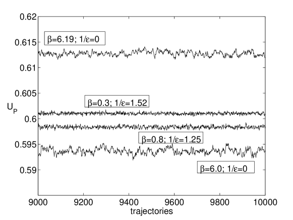
Figure 8: Comparison of short portions of plaquette histories for different combinations of $\beta$ and $\varepsilon$.

Of course, such tests should be extended to further observables, but our results for the plaquette value are encouraging.

5 Conclusions

The conservation of the topological charge can be implemented in the lattice gauge action to some extent. There are various obstacles preventing a strict implementation, such as scaling artifacts and the acceptance rate. Still, we succeeded in obtaining long sequences of a stable topological charge, although it cannot be fixed strictly, as expected. Our comparison to the behaviour of the plaquette value suggests that the topological autocorrelation time exceeds by far the autocorrelation of other observables. This property facilitates the collection of many configurations in a specific topological sector, for actions which are perfectly acceptable. We also observed that such actions do not seem to suffer from any conceptual problems. In particular the resulting static potential is fully consistent with the right continuum limit, and it has relatively mild lattice artifacts. We also showed that at least a positive squared transfer matrix can be defined.

Moreover we found benefits of this action for the kernel condition number of the overlap operator, which allows for a somewhat faster evaluation with a fixed accuracy. We finally remark that our findings are in accordance with recent results of Refs. [36]. Further virtues, in particular in view of the simulations with dynamical quarks, still remain to be explored.

Acknowledgement    We would like to thank M. Creutz, H. Fukaya, S. Hashimoto, M. Ilgenfritz, M. Lüscher, M. Müller-Preußker, K. Ogawa, T. Onogi, R. Sommer and C. Urbach for interesting discussions and helpful remarks. This work was supported by the “Deutsche Forschungsgemeinschaft” through SFB/TR9-03. S. Necco is supported by TMR, EC-Contract No. HPRNCT-2002-00311 (EURIDICE). Part of the computations were performed on the IBM p690 clusters of the “Norddeutscher Verbund für Hoch- und Höchstleistungsrechnen” (HLRN) and at the Forschungszentrum Jülich.

References

- [1] K.G. Wilson, Phys. Rev. D10 (1974) 2445.
- [2] I. Montavay and G. Münster, “Quantum Fields on the Lattice”, Cambridge University Press (Cambridge UK, 1994).
- [3] P. Weisz, Nucl. Phys. B212 (1983) 1.
- [4] M. Lüscher and P. Weisz, Phys. Lett. B158 (1985) 250; Commun. Math. Phys. 97 (1985) 59.
- [5] Y. Iwasaki, UTHEP-118. Y. Iwasaki and T. Yoshié, Phys. Lett. B143 (1984) 449.
- [6] P. DeForcrand et al. (QCDTARO Collaboration), Nucl. Phys. (Proc. Suppl.) B53 (1997) 938. T. Takaishi, Phys. Rev. D54 (1996) 1050.
- [7] F. Niedermayer, P. Rüfenacht and U. Wenger, Nucl. Phys. B597 (2001) 413.
- [8] M. Lüscher, hep-lat/0409106, hep-lat/0509152. C. Urbach, K. Jansen, A. Shindler and U. Wenger, hep-lat/0506011.
- [9] S. Weinberg, Physica A96 (1979) 327. J. Gasser and H. Leutwyler, Ann. Phys. (N.Y.) 158 (1984) 142.
- [10] P.H. Ginsparg and K.G. Wilson, Phys. Rev. D25 (1982) 2649.
- [11] P. Hasenfratz, V. Laliena and F. Niedermayer, Phys. Lett. B427 (1998) 125. P. Hasenfratz, Nucl. Phys. B525 (1998) 401.
- [12] M. Lüscher, Phys. Lett. B428 (1998) 342.
- [13] H. Neuberger, Phys. Lett. B417 (1998) 141; Phys. Lett. B427 (1998) 353.
- [14] J. Gasser and H. Leutwyler, Phys. Lett. B184 (1987) 83.
- [15] J. Gasser and H. Leutwyler, Phys. Lett. B188 (1987) 477. H. Neuberger, Phys. Rev. Lett. 60 (1988) 889; Nucl. Phys. B300 (1988) 180. P. Hasenfratz and H. Leutwyler, Nucl. Phys. B343 (1990) 241. F.C. Hansen, Nucl. Phys. B345 (1990) 685. F.C. Hansen and H. Leutwyler, Nucl. Phys. B350 (1991) 201. W. Bietenholz, Helv. Phys. Acta 66 (1993) 633.
- [16] H. Leutwyler and A. Smilga, Phys. Rev. D46 (1992) 5607. P.H. Damgaard et al., Nucl. Phys. B629 (2002) 445, Nucl. Phys. B656 (2003) 226.
- [17] S. Prelovsek and K. Orginos, Nucl. Phys. (Proc. Suppl.) B119 (2003) 822.
- [18] W. Bietenholz, K. Jansen and S. Shcheredin, JHEP 07 (2003) 033. L. Giusti, M. Lüscher, P. Weisz and H. Wittig, JHEP 11 (2003) 023. D. Galletly et al., Nucl. Phys. (Proc. Suppl.) B129/130 (2004) 456.
- [19] L. Giusti, M. Lüscher, P. Weisz and H. Wittig, JHEP 0311 (2003) 023. L. Del Debbio and C. Pica, JHEP 0402 (2004) 003. L. Del Debbio, L. Giusti and C. Pica, Phys. Rev. Lett. 94 (2005) 032003.
- [20] W. Bietenholz, T. Chiarappa, K. Jansen, K.-I. Nagai, and S. Shcheredin, JHEP 02 (2004) 023.
- [21] L. Giusti, P. Hernández, M. Laine, P. Weisz and H. Wittig, JHEP 01 (2004) 003.
- [22] L. Giusti, P. Hernández, M. Laine, P. Weisz and H. Wittig, JHEP 04 (2004) 013. L. Giusti and S. Necco, PoS(LAT2005)132 [hep-lat/0510011].
- [23] S. Shcheredin, Ph.D. thesis (Berlin, 2004) [hep-lat/0502001]. W. Bietenholz and S. Shcheredin, Rom. J. Phys. 50 (2005) 249 [hep-lat/0502010]; PoS(LAT2005)138 [hep-lat/0508016]. S. Shcheredin and W. Bietenholz, PoS(LAT2005)134 [hep-lat/0508034].
- [24] H. Fukaya, S. Hashimoto and K. Ogawa, Prog. Theor. Phys. 114 (2005) 451; PoS(LAT2005)134 [hep-lat/0510049]. K. Ogawa and S. Hashimoto, Prog. Theor. Phys. 114 (2005) 609.
- [25] J. Wennekers and H. Wittig, JHEP 0509 (2005) 059. L. Giusti, P. Hernández, M. Laine, C. Pena, J. Wennekers and H. Wittig, PoS(LAT2005)344 [hep-lat/0510033].
- [26] P.H. Damgaard and S.M. Nishigaki, Nucl. Phys. B518 (1998) 495; Phys. Rev. D63 (2001) 045012.
- [27] K. Orginos, Nucl. Phys. (Proc. Suppl.) 106 (2002) 721. Y. Aoki et al., Phys. Rev. D69 (2004) 074504.
- [28] P. Hernández, K. Jansen and M. Lüscher, Nucl. Phys. B552 (1999) 363.
- [29] H. Neuberger, Phys. Rev. D61 (2000) 085015.
- [30] K. Nagao, hep-th/0509034.
- [31] M. Lüscher, Nucl. Phys. B549 (1999) 295; Nucl. Phys. B568 (2000) 162.
- [32] H. Fukaya and T. Onogi, Phys. Rev. D68 (2003) 074503; Phys. Rev. D70 (2004) 054508.
- [33] M. Creutz, Phys. Rev. D70 (2004) 091501.
- [34] S. Shcheredin, W. Bietenholz, K. Jansen, K.-I. Nagai, S. Necco and L. Scorzato, Nucl. Phys. (Proc. Suppl.) B140 (2005) 779 [hep-lat/0409073]. W. Bietenholz, K. Jansen, K.-I. Nagai, S. Necco, L. Scorzato and S. Shcheredin, AIP Conf. Proc. 756 (2005) 248 [hep-lat/0412017]. K.-I. Nagai, K. Jansen, W. Bietenholz, L. Scorzato, S. Necco and S. Shcheredin, PoS(LAT2005)283 [hep-lat/0509170].
- [35] H. Fukaya, T. Onogi, S. Hashimoto, T. Hirohashi and K. Ogawa, PoS(LAT2005)134 [hep-lat/0509184].
- [36] H. Fukaya, S. Hashimoto, T. Hirohashi, H. Matsufuru, K. Ogawa, and T. Onogi, PoS(LAT2005)123 [hep-lat/0510095]. H. Fukaya, S. Hashimoto, T. Hirohashi, K. Ogawa, and T. Onogi, hep-lat/0510116.
- [37] P. Marenzoni, L. Pugnetti and P. Rossi, Phys. Lett. B315 (1993) 152.
- [38] M. Albanese et al., Phys. Lett. 192B (1987) 163.
- [39] M. Guagnelli, R. Sommer and H. Wittig, Nucl. Phys. B535 (1998) 389.
- [40] S. Necco and R. Sommer, Nucl. Phys. B622 (2002) 328.
- [41] R. Sommer, Nucl. Phys. B411 (1994) 839.
- [42] S. Necco, Nucl. Phys. B683 (2004) 137; Ph.D. thesis (Berlin, 2004) [hep-lat/0306005].
- [43] H. Grosse and H. Kuhnelt, Nucl. Phys. B205 (1982) 273.
- [44] N. Manton, Phys. Lett. B96 (1980) 328.
- [45] W. Bietenholz, Eur. Phys. J. C6 (1999) 537; Nucl. Phys. B644 (2002) 223. W. Bietenholz and I. Hip, Nucl. Phys. B570 (2000) 423 [hep-lat/9902019]. T. DeGrand, Phys. Rev. D63 (2001) 034503. W. Kamleh, D.H. Adams, D.B. Leinweber and A.G. Williams, Phys. Rev. D66 (2002) 014501. S. Dürr, C. Hoelbling and U. Wenger, hep-lat/0506027.
- [46] E.-M. Ilgenfritz, M.L. Laursen, G. Schierholz, M. Müller-Preußker and H. Schiller, Nucl. Phys. B268 (1986) 693.