BULK THERMODYNAMICS OF $SU(N)$ LATTICE GAUGE THEORIES AT LARGE-$N$

Abstract

We present a study of bulk thermodynamical quantities in the deconfined phase of pure lattice $SU(N)$ gauge theories. We find that the deficit in pressure and entropy with respect to their free-gas values, for $N=4,8$, is remarkably close to that of $SU(3)$. This suggests that understanding the strongly interacting nature of the deconfined phase, which is crucial for RHIC physics, can be done at large $N$. There, different analytical approaches simplify or become soluble, and one can check their predictions and point to their important ingredients.

1 Introduction

Recent discoveries at RHIC point to the inadequacy of using a weakly coupled plasma description for the deconfined phase of QCD (see for example [1] and references therein). Instead, properties of collective flow, can be described very well with ideal hydrodynamics, which suggests that the phase is in fact strongly interacting. Related to these are theoretical studies in the framework of lattice QCD, which found signs of these strong interactions. These include a large deficit in thermodynamical bulk properties, such as pressure, entropy, and energy density, with respect to their free gas values, up to temperatures of a few times the transition temperature $T_{c}$ [2] . These deficits were found in the pure $SU(3)$ gauge theory, as well as with different types of fermions. The deficit in all these cases is quite similar, and is hard to reproduce with standard perturbation theory. This is in contrast to the fermionic addition to the pressure at a small, nonzero, chemical potential, which is explained very well by perturbation theory (for example [4] and references thererin).

The analytical approaches used to study this phenomenon include quasi-particle models, Polyakov loop models, variants of perturbation theory, models of loosely bound states, gravity dual models, and also perturbative small volume calculations of the large-$N$ gauge theory. Some of these approaches simplify or even become soluble at the ‘t Hooft limit of large-$N$, which is a free theory in the confined phase (at least in the mesonic sector), and consists of only planar diagrams in a perturbative expansion of the deconfined phase. An additional important point here is that, provided the chiral limit is taken after the large-$N$ limit, the planar pure gauge theory is effectively quenched (for example see [5]). This makes any calculation in the pure gauge case relevant for the physical case, that includes fermions.

The simplifications of the planar limit, together with the possibility that the pressure deficit is ‘hidden’ in the gluonic sector, and the need to check and constraint the analytical explanations, lead us to study bulk thermodynamical properties of $SU(4)$, and $SU(8)$ pure lattice gauge theories and compare to the study by Boyd et al. of $SU(3)$ [2]. Recent calculations of various properties of $SU(N)$ gauge theories [6]–[10] have demonstrated that $N=8$ is very close to $N=\infty$ for most purposes. These also provide information on the transition coupling for various lattice sizes and $N$. Thus our calculations should provide us with an accurate picture of what happens to bulk thermodynamics at $N=\infty$. For a more detailed version of this work, which was conducted with Dr. M. Teper, we refer to [11].

2 Lattice setup and methodology

We define the gauge theory on a discretised periodic Euclidean four dimensional space-time with $L^{3}_{s}\times L_{t}$ sites, and perform Monte-Carlo simulations of a simple Wilson action. We use the Kennedy-Pendelton heat bath algorithm for the link updates, followed by five over-relaxations of all the $SU(2)$ subgroups of $SU(N)$. To evaluate bulk thermodynamics there are several approaches one can use. The “differential method” was used in the past, and is known to produce the unphysical result of a negative pressure close to $T_{c}$. The reason for that is the use of a perturbative beta function in a regime where the coupling is not small. In our case, larger values of $N$ drive us to smaller values of $L_{t}=5$, and therefore to a lattice spacing of $a\simeq 1/(5T_{c})$- too coarse for the differential method. An additional possibility is the use of a direct evaluation of the density of states. Unfortunately, modern methods like the Wang-Landau algorithm did not converge for the case of $SU(8)$. This leaves us with the “integral method” (see for example [2]) in which the pressure $p$ and interaction measure $\Delta$ are

$$p/T^{4}=6L^{4}_{t}\int^{\beta}_{\beta_{0}}d\beta^{\prime}(\langle u_{p}\rangle_{T}-\langle u_{p}\rangle_{0}),\qquad\Delta/T^{4}=6L_{t}^{4}(\langle u_{p}(\beta)\rangle_{0}-\langle u_{p}(\beta)\rangle_{T})\times\frac{\partial\beta}{\partial\log(a(\beta))}.$$ (1)

Here $\langle u_{p}\rangle_{T}$ is the plaquette average on a $T>0$ lattice with $L_{t}<L_{s}$, while $\langle u_{p}\rangle_{0}$ is measured on a lattice with relatively large $L_{t}=L_{s}$. Let us mention that in the expression for the pressure in Eq. (1) we dropped the pressure at temperature $T_{0}$ corresponding to $\beta_{0}$. To justify this one usually takes $\beta_{0}$ much lower than the transition coupling $\beta_{c}$, which means that the systematic error will be very small.

We performed calculations of $\langle u_{p}\rangle_{T}$ in $SU(4)$ on $16^{3}5$ lattices and in $SU(8)$ on $8^{3}5$ lattices for a range of $\beta$ values corresponding to $T/T_{c}\in[0.89,1.98]$ for $SU(4)$, and to $T/T_{c}\in[0.97,1.57]$ for $SU(8)$. Since we use $L_{t}=5$, while the data for $SU(3)$ in [2] is for $L_{t}=4,6,8$, we also performed simulations for $SU(3)$ on $20^{3}5$ lattices with $T/T_{c}\in[1,2]$. The measured plaquette averages are presented in [11].

We performed the ‘$T=0$’ calculations of $\langle u_{p}\rangle_{0}$ on $20^{4}$ lattices for SU(3), and on $16^{4}$ lattices for SU(4), which are known to be effectively at $T=0$ [9, 10] for the couplings involved. For SU(8) however, using $8^{4}$ lattices would not be adequate for the largest $\beta$-values, and we take instead the SU(8) calculations on larger lattices in [10], and interpolate between the values of $\beta$ used there with the ansatz $\langle u_{p}\rangle_{0}(\beta)=\langle u_{p}\rangle^{P.T.}_{0}(\beta)+\frac{\pi^{2}}{12}\frac{G_{2}}{N\sigma^{2}}(a\sqrt{\sigma})^{4}+c_{4}g^{8}+c_{5}g^{10},$ where $\langle u_{p}\rangle^{P.T.}_{0}(\beta)$ is the lattice perturbative result to ${\cal O}(g^{6})$ from [12] and $N=8$. Our best fit has $\chi^{2}/{\rm dof}=0.93$ with ${\rm dof}=2$, and the best fit parameters are $c_{4}=-6.92$, $c_{5}=26.15$, and a gluon condensate of $\frac{G_{2}}{N\sigma^{2}}=0.72$.

3 Finite volume effects

For $N=4,8$, one is able to use lattice volumes much smaller than what one needs for $SU(3)$ (like those in [2]) as the longest correlation length decreases rapidly with $N$ [7, 8]. This is also theoretically expected, much more generally, as $N\to\infty$ (see for example [5]). The main remaining concern has to do with tunneling configurations, which occur only at $T_{c}$ when $V\to\infty$. On our finite volumes, this is no longer true, and we minimise finite-$V$ corrections by calculating the average plaquettes only in field configurations that are confining, for $T<T_{c}$, or deconfining, for $T>T_{c}$. For SU(3), where the phase transition is only weakly first order, it is not practical to attempt to separate phases. This will smear the apparent variation of the pressure across $T_{c}$ in the case of SU(3).

To confirm that our finite volume effects are under control we have compared the SU(8) value of $\langle u_{p}(\beta)\rangle$ as measured in the deconfined phase of the our $8^{3}\times 5$ lattice with other $L_{s}^{3}\times 5$ results from other studies [13], and find that the results are consistent at the $2$ sigma level. We perform a similar check for the confined phase on the same lattices, and again find that finite volume effects are small, mostly on a one sigma level. A similar check for the confined phase on $L^{4}$ lattices leads to conclude that a size $L=8$ in SU(8) is not large enough, as we find that the plaquette average has a significant change (on a $16$ sigma level) from $L=8$ to $L=16$ for our largest value of $\beta$. By contrast, for $SU(4)$ the finite volume effects seem not to be large on the $16^{4}$ lattice as we checked for our largest value of $\beta=11.30$. There the value of the plaquette on a $20^{4}$ lattice is consistent within $\sim 2.3$ sigma with the value on a $16^{4}$ lattice. The data supporting these checks, together with the checks related to the next paragraph, is presented in [11].

4 Finite lattice spacing corrections

To evaluate the scaling of the temperature $T$ with the coupling $\beta=2N/g^{2}$, and the derivative in Eq. (1), we use calculations of the string tension, $\sigma$, in lattice units (e.g. [8]). A more natural scale here is the transition temperature $T_{c}$. However this involves a calculation of the transition coupling $\beta_{c}$ for many values of $L_{t}$, and for several values of $L_{s}$, which is a very large scale project. Also the difference between this scale fixing and the one according to $\sigma$ comes from the $O(a^{2})$ corrections of $T_{c}/\sqrt{\sigma}$. A check of the latter for $SU(3),SU(8)$ shows that $T_{c}/\sqrt{\sigma}$ for $L_{t}=5,8$, are the same within the errors. Indeed when we compare $T/T_{c}(\beta)$ from [2], and as determined here for $N=3$, we find that they fall on top of each other. This is not the case for $SU(4)$, but there the $5\sigma$ difference in $T_{c}/\sqrt{\sigma}$ of $L_{t}=5$, and $L_{t}=8$ is only at the level of $2\%$. As a result we may slightly overestimate $T/T_{c}$ when it is $\sim 8/5$ for this $N=4$. Finally the value of $T_{c}/\surd\sigma$ for the different gauge groups and $L_{t}=5$ in taken from [7, 8].

In presenting our results for the pressure, we shall normalize to the lattice Stephan-Boltzmann result given by $\left(p/T^{4}\right)_{\rm{free-gas}}=(N^{2}-1)\frac{\pi^{2}}{45}\times R_{I}(L_{t}).$ Here $R_{I}$ includes the effects of discretization errors in the integral method [14, 11]. The same normalisation is applied for the interaction measure $\Delta$, and for the energy density $\epsilon=\Delta+3p$, and entropy density $s=(\Delta+4p)/T$.

To check that we understand the systematics of finite lattice spacing corrections when presenting the normalized results, we compare $\Delta/T^{4}$ for $SU(3)$ with $L_{t}=4,6$ from [2], $L_{t}=5$ from the current study (in both these cases $T$ was increased by increasing $\beta$), and $L_{t}=2,3,4$ from [8] (where $T$ was increased by decreasing $L_{t}$). The result of the comparison is presented in the left panel of Fig. 1, where one indeed sees that the normalization by the Stephan-Boltzmann free gas shows a systematic increase of $\Delta$ towards the continuum limit.

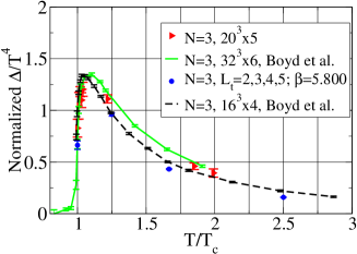
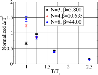
Figure 1: $\Delta$ for $N=3$ (on the left), and $N=3,4,8$ (on the right) normalized to the lattice Stephan-Boltzmann pressure, including the full discretization errors given by $R_{I}$. The lines are the $SU(3)$ results and $L_{t}=4,6$ from [2].

5 Results

Before we present our results for the bulk thermodynamical quantities, let us note that as the ideas of reduction at large-$N$ (for example see the recent systematic studies in [5]) have an interesting realization here. By relabeling the axes, the authors of [15] have argued that at $N=\infty$ Wilson loops should not change as a function of $T$ for $T<T_{c}$. This will be reflected in our case in a $\langle u_{p}\rangle_{T=T_{c}^{-}}$ which is very similar to $\langle u_{p}\rangle_{0}$. Indeed when we compare the two we find that the difference is on a $\sim 2\sigma$ level for $SU(4),SU(8)$, while from the data of [14] it is on the $15\sigma$ level for $SU(3)$. This also means that the systematic error, ignored in Eq. (1) is very small for the larger values of $N$.

All the results we present are as a function of $T/T_{c}$. It is therefore important to note that the dependence of $T_{c}$ on $N$ is very weak, indeed like many other quantities in the pure gauge theory [16]. We present our $N=4$ and $N=8$ results for $\Delta/T^{4}$ in the right panel of Fig. 1, and on Fig. 2. In the former we change $L_{t}$ so to increase $T$ up to $T=2.5T_{c}$, while in the latter $T$ is increased by changing $\beta$. In both cases we find modest/small changes between the different groups. Nonetheless in the vicinity of $T_{c}$, the differences are large, presumably because the transition in $SU(3)$ is only weakly first order.

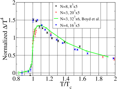
Figure 2: $\Delta/T^{4}$ normalized to the lattice Stephan-Boltzmann pressure, including the full discretization errors given by $R_{I}$, for $N=3,4,8$. The line are the $SU(3)$ results and $L_{t}=6$ from [2]

.

The plot of $p/T^{4}$ is presented in the left panel of Fig. 3. We also show our calculations of the $SU(3)$ pressure for $L_{t}=5$, as well as the $L_{t}=6$ calculations from [2]. In the right panel of Fig. 3 we present results for the normalized energy density $\epsilon$, and normalized entropy density $s$. The lines are the $SU(3)$ result of [2] with $L_{t}=6$. Again we see very little dependence on the gauge group, implying very similar curves for $N=\infty$.

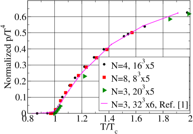
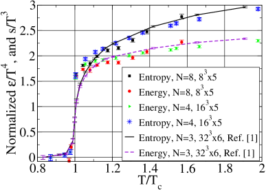
Figure 3: The pressure (on the left), and energy and entropy densities (on the right) normalized to the lattice Stephan-Boltzmann pressure, including the full discretization errors given by $R_{I}$. In the pressure plot, the symbols’ vertical sizes are representing the largest error bars (which are received for the highest temperature). The lines are the $SU(3)$ results and $L_{t}=6$ from [2].

One can clearly infer that the pressure in the $SU(4)$ and $SU(8)$ cases is remarkably close to that in $SU(3)$ and hence that the well-known pressure deficit observed in SU(3) is in fact a property of the large-$N$ planar theory. This implies that the dynamics that drives the deconfined system far from its noninteracting gluon gas limit, must remain equally important in the $N=\infty$ planar theory. This is encouraging since this limit is simpler to approach analytically, for example using gravity duals, and also because it can serve to constraint and point to important ingredients of analytical approaches. For example, in perturbation theory, it tells us that the important contributions must be planar, and although the current calculated contributions are indeed all planar, this is not guaranteed at $O(g^{7})$ [17]. In models focusing on resonances and bound states, it must be that the dominant states are coloured, since the contribution of colour singlets will vanish as $N\to\infty$. Models using ‘quasi-particles’ should place these in colour representations that do not exclude their presence at $N=\infty$, and in fact give them $T$-dependent properties which depend weakly on $N$. Also, topological fluctuations should play no role in this deficit since the evidence is that there are no topological fluctuations of any size in the deconfined phase at large-$N$ [18, 19].

References

- [1] U. W. Heinz, J. Phys. G 31, S717 (2005) [arXiv:nucl-th/0412094]. E. V. Shuryak, Nucl. Phys. A 750, 64 (2005) [arXiv:hep-ph/0405066].
- [2] G. Boyd, J. Engels, F. Karsch, E. Laermann, C. Legeland, M. Lutgemeier and B. Petersson, Nucl. Phys. B 469, 419 (1996) [arXiv:hep-lat/9602007].
- [3] P. Petreczky, Nucl. Phys. Proc. Suppl. 140, 78 (2005) [arXiv:hep-lat/0409139].
- [4] P. de Forcrand, these proceedings.
- [5] R. Narayanan and H. Neuberger, arXiv:hep-lat/0509014.
- [6] B. Lucini, M. Teper and U. Wenger, Phys. Lett. B 545, 197 (2002) [arXiv:hep-lat/0206029].
- [7] B. Lucini, M. Teper and U. Wenger, JHEP 0401, 061 (2004) [arXiv:hep-lat/0307017].
- [8] B. Lucini, M. Teper and U. Wenger, JHEP 0502, 033 (2005) [arXiv:hep-lat/0502003].
- [9] B. Lucini and M. Teper, JHEP 0106, 050 (2001) [arXiv:hep-lat/0103027].
- [10] B. Lucini, M. Teper and U. Wenger, JHEP 0406, 012 (2004) [arXiv:hep-lat/0404008].
- [11] B. Bringoltz and M. Teper, Phys. Lett. B 628, 113 (2005) [arXiv:hep-lat/0506034].
- [12] B. Alles, A. Feo and H. Panagopoulos, Phys. Lett. B 426, 361 (1998) [Erratum-ibid. B 553, 337 (2003)] [arXiv:hep-lat/9801003].
- [13] B. Bringoltz and M. Teper, arXiv:hep-lat/0508021.
- [14] J. Engels, F. Karsch and T. Scheideler, Nucl. Phys. B 564, 303 (2000) [arXiv:hep-lat/9905002]. J. Engels, private Communications (2005)
- [15] A. Gocksch and F. Neri, Phys. Rev. Lett. 50, 1099 (1983).
- [16] M. Teper, arXiv:hep-lat/0509019.
- [17] Y. Schroder, private communications (2005).
- [18] B. Lucini, M. Teper and U. Wenger, Nucl. Phys. B 715, 461 (2005) [arXiv:hep-lat/0401028].
- [19] L. Del Debbio, H. Panagopoulos and E. Vicari, JHEP 0409, 028 (2004) [arXiv:hep-th/0407068].