Chiral and Continuum Extrapolation of Partially-Quenched Hadron Masses

Abstract:

Using the finite-range regularisation (FRR) of chiral effective field theory, the chiral extrapolation formula for the vector meson mass is derived for the case of partially-quenched QCD. We re-analyse the dynamical fermion QCD data for the vector meson mass from the CP-PACS collaboration. A global fit, including finite lattice spacing effects, of all 16 of their ensembles is performed. We study the FRR method together with a naive polynomial approach and find excellent agreement ($\sim 1$%) with the experimental value of $M_{\rho}$ from the former approach. These results are extended to the case of the nucleon mass.

PoS(LAT2005)049

1 Introduction

Current computers and algorithms enable lattice gauge theorists to perform simulations of QCD over a relatively wide range of parameters, even in the dynamical-fermion case. However, despite the enormous progress made, physical values of the light quark masses are still not within reach. In order for the lattice to make predictions at these quark masses, a chiral extrapolation procedure is inevitable.

The traditional (dimensional regularised) chiral perturbation theory approach is well known to suffer from convergence problems. As a symptom of this, very poor agreement is found when lattice data is fitted to a truncated (dim-reg) chiral series using the known values of the non-analytic (in quark mass) coefficients [1]. This situation can be understood on physical grounds due to the fact that chiral perturbation theory is an effective theory. When effective theories are applied beyond their range of validity, more and more interaction terms are typically required to mop up for the physics that the effective theory intrinsically misses. Such a situation occurs in the case of chiral perturbation theory as the quark mass becomes moderate. In this case, as the light quantum fields (i.e. the pions) become massive and their Compton wavelengths decrease in size, they begin to probe the quark nature underlying the hadronic fields in the effective theory. The chiral effective theory therefore breaks down.

Fortunately we have comprehensive lattice data over a wide range of quark masses in the region where the chiral perturbation theory is no longer valid. This data tells us that the hadonic masses are typically very linear in the quark mass, $m_{q}$, for $m_{q}\;\raisebox{-2.15277pt}{\hbox to0.0pt{$\sim$\hss}}\raisebox{2.15277pt}{$>$}\;m_{s}/2\approx 50$ MeV.

The aim of using chiral extrapolation techniques is therefore to respect both the properties of the effective theory at small $m_{q}$, and the lattice data at moderate to large $m_{q}$. The finite-range regulator (FRR) or Adelaide approach to chiral effective theory provides such a method. In this approach, a scale, $\Lambda$, is introduced representing the transition scale where pion interaction effects should be moderated. This scale is introduced naturally in a form factor for the pion-hadron interactions. In this formalism, pion loops are moderated like $\Lambda\!/\!m_{q}$ as $m_{q}$ grows, and FRR reproduces (by construction) the structure of traditional dim-reg chiral effective theory in the $m_{q}\rightarrow 0$ limit. The FRR approach therefore provides a marriage between chiral effective theory and lattice data.

In this talk, we extend previous FRR work to the vector meson mass in the “partially-quenched” case (i.e. when $m_{q}^{sea}\neq m_{q}^{val}$). This method is then applied to a dataset from the CP-PACS Collaboration [4]. An extension of this work to the partially-quenched nucleon mass is also briefly discussed. A full description of this work can be found in [2, 3]

2 The FRR Approach

We introduce the nomenclature $M_{V(PS)}(\beta,s;v_{1},v_{2})$ for the vector (pseudoscalar) meson mass calculated with a gauge coupling of $\beta$, sea quark mass of $s$, and valence quark masses of $v_{1}$ and $v_{2}$.

The FRR expression for the vector mass is [2, 3]

$$M_{V}^{2}(\beta,s;v,v)=(a_{0}+a_{2}M^{2}_{PS}(\beta,s;v,v)+a_{4}M^{4}_{PS}(\beta,s;v,v)+\ldots)^{2}+\Sigma_{TOT}$$ (1)

$$\mbox{where }\;\;\;\;\;\;\Sigma_{TOT} = \Sigma^{\rho}_{\pi\pi}(M^{2}_{PS}(\beta,s;s,v))+\Sigma^{\rho}_{\pi\omega}(M^{2}_{PS}(\beta,s;s,v))$$

$$+ \Sigma_{DHP}(M^{2}_{PS}(\beta,s;s,v),M^{2}_{PS}(\beta,s;v,v),M^{2}_{PS}(\beta,s;s,s)).$$

Note that we derive this expression for vector mesons composed only of degenerate valence quarks.

The $\Sigma$ terms are self-energies and are diagrammatically depicted in Fig. 1 of [2]. We give below the definition of $\Sigma^{\rho}_{\pi\omega}$; see [2] for expressions for $\Sigma^{\rho}_{\pi\omega}$ and $\Sigma_{DHP}$.

$${\Sigma^{\rho}_{\pi\omega}} = -\frac{g_{\omega\rho\pi}^{2}\mu_{\rho}}{12\pi^{2}}\int_{0}^{\infty}\frac{k^{4}u_{\pi\omega}^{2}(k)~{}dk}{\omega_{\pi}^{2}(k)}$$

$$\mbox{with }\;\;\;\;\;\;\;\omega_{\pi}^{2}(k) = k^{2}+M^{2}_{PS}(\beta,s;s,v)\;\;\;\;\;\mbox{and }\;\;\;\;\;\;\;u(k)=\frac{\Lambda^{4}}{(\Lambda^{2}+k^{2})^{2}}.$$

Here $g_{\omega\rho\pi}\mu_{\rho}$ defines the coupling of $\rho\to\omega\pi$ with $g_{\omega\rho\pi}=16$ GeV^-1 and the physical $\rho-$mass $\mu_{\rho}=770$ MeV. The form factor $u(k)$ has a natural scale, $\Lambda$, which was referred to in the previous section. Finally note that Eq. (1) reproduces dim-reg $\chi$PT as $M_{\pi}\rightarrow 0$.

The momentum integrals in the $\Sigma$ definitions are discretised to the lattice using

$$4\pi\int_{0}^{\infty}k^{2}dk=\int d^{3}k\approx\frac{1}{V}\left(\frac{2\pi}{a}\right)^{3}\sum_{k_{x},k_{y},k_{z}}$$

with $k_{\mu}$ being constrained by the finite periodic volume of the lattice.

3 CP-PACS Data

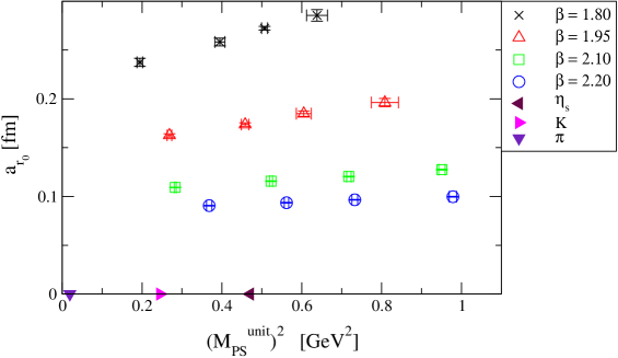
Data for the vector meson mass was taken from the CP-PACS Collaboration [4]. These simulations used two-flavours of mean-field improved Wilson fermions with Iwasaki glue. There is, therefore, the possibility of some residual ${\cal O}(a)$ systematics. The CP-PACS dataset comprises of four different $\beta$’s, with four $\kappa^{\rm sea}$ values for each $\beta$ value, making a total of 16 independent ensembles. In addition, each ensemble has five different valence quarks, meaning that there are a total of 80 (degenerate) meson masses. We represent each of these masses by a 1000-element bootstrap ensemble which is Gaussianly-distributed about the CP-PACS central value with the FWHM set to the quoted error in [4]. The parameter space spanned by this CP-PACS dataset is displayed in Fig. 1.

Figure 1: CP-PACS parameter range in lattice spacing, $a$ (from $r_{0}$) and $M_{PS}^{unit}$, where “unit” refers to the unitary point (i.e. $m_{q}^{sea}=m_{q}^{val}$). The physical light pseudoscalar mesons are included for reference.

4 Fitting Procedure

The procedure used to fit the CP-PACS data to the FRR functions is as follows. Prior to the extrapolation, we first convert all masses into physical units using both the string tension, and hadronic scale, $r_{0}$. This has the following two advantages compared to an analysis with dimensionless hadron masses: different ensemble’s data can be combined together in a global fit; and since dimensionful mass predictions from lattice simulations are ratios of lattice mass estimates, some systematic and statistical errors will cancel.

We then use the FRR functional form below to fit the data.

$$\sqrt{M_{V}^{2}(\beta,s;v,v)\!-\!\Sigma_{TOT}}\!=\!(a^{cont}_{0}\!\!\!+\!X_{1}a\!+\!X_{2}a^{2})\!+\!a_{2}M^{2}_{PS}(\beta,s;\!v,v)\!+\!a_{4}M^{4}_{PS}(\beta,s;\!v,v)\!+\!a_{6}M^{6}_{PS}(\beta,s;\!v,v).$$ (2)

This is simply Eq. (1) modified by the addition of ${\cal O}(a,a^{2})$ terms to the $a_{0}$ coefficient in order to model the lattice spacing systematics. We tested the addition of terms ${\cal O}(a,a^{2})$ to the $a_{2,4,6}$ coefficients as well, but found that these terms were either compatible with zero, or lead to unstable fits. Variants of Eq. (2) were used to study the stability of the fit procedure: including the $X_{1}a$ term, or alternatively setting $X_{1}\equiv 0$; and including the “cubic” $a_{6}M_{PS}^{6}$ term, or alternatively setting $a_{6}\equiv 0$ (the “quadratic” fit).

As well as the FRR function in Eq. (2), we fitted the data to a naive polynomial fit function defined by Eq. (2) but with $\Sigma_{TOT}$ set to zero (labelled as Naive in the following).

The above fitting functions were used in a “global” fit of all the CP-PACS data. Since there are 80 meson mass datapoints (see Sec. 3) a highly constrained fit was obtained since the number of fitting parameters is tiny compared to 80. See [2, 3] for details of the fit procedure

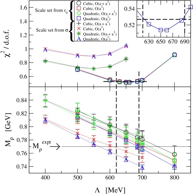
Recall that in the case of the FRR fit, an extra parameter, $\Lambda$ is introduced to govern the sum of higher-order terms of the expansion with guidance from lattice QCD data. We find that $\Lambda$ is constrained well by the large CP-PACS data set. Figure 2 (upper plot) shows the behaviour of the $\chi^{2}$ for the above FRR fits. Results for the four variants to Eq. (2) as discussed above are shown. The insert shows the result for the preferred fitting function choice (which is $X_{1}\equiv 0$ and $a_{6}\equiv 0$, see [3]). By increasing $\chi^{2}$ by one from its minimum value, we obtain the acceptable range of $\Lambda=655(35)$ MeV.

Figure 2: Upper: $\chi^{2}/d.o.f.$ versus the FRR $\Lambda$ parameter. (The insert shows a close up of the $\chi^{2}$ minimum region.) Lower: $M_{\rho}$ prediction versus $\Lambda$. The vertical dashed lines represent $\Lambda=655(35)$ MeV.

We find that the FRR approach gives lower $\chi^{2}$ values than the naive polynomial fits; that the chiral series (in the FRR approach) is very convergent (i.e. the inclusion of the ${\cal O}(M_{PS}^{6})$ term is irrelevant in these fits); and that $r_{0}$ is a more stable quantity to set the scale than the string tension.

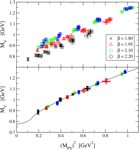
The success of the FRR approach in fitting the data can be seen in Fig. 3 by comparing the raw CP-PACS data in the upper plot with the data corrected according to Eq. (2) in the lower plot.

Figure 3: Upper: The raw 80 CP-PACS data. Lower: The same data after correction according to Eq. (4.1).

5 $M_{\rho}$ and $M_{n}$ estimate

The final value estimate for $M_{\rho}$ is obtained using the $a_{0,2,4}$ parameters from the fit, and by setting $a=0$, and $M_{PS}$ to the physical pion mass. We obtain

$$M_{\rho}^{FRR}=778(4){\scriptstyle{}^{+{13}}_{-{0}}}{\scriptstyle{}^{+{8}}_{-{9}}}\;\;\textrm{MeV}\;\;\;\;\;\mbox{and}\;\;\;\;\;M_{\rho}^{Naive}=825(4){\scriptstyle{}^{+{12}}_{-{8}}}\;\;\textrm{MeV}$$ (3)

where the errors are statistical, fit procedure, and, in the FRR case, from the variation in $\Lambda$. This last error is obtained from the lower plot in Fig. 2, where the variation of the $M_{\rho}$ prediction as a function of $\Lambda$ is shown. Using the range $\Lambda=655(35)$ MeV (see Sec. 4) we obtain the third error.

Note that we do not include an error estimate due to the uncertainty in $r_{0}$ itself, nor from the fact that the number of dynamical flavours, $N_{f}\neq 2+1$.

As can be seen the errors from the various sources are typically around 1%, including the uncertainty due to the $\Lambda$ value. Note also that the FRR $M_{\rho}$ estimate is in comfortable agreement with the experimental value (in contrast with the naive polynomial fit).

In [4], nucleon mass data was also published. The FRR formula for the partially-quenched nucleon case was derived and a similar fitting procedure to that outlined here for the vector case was applied. The estimate of the nucleon mass from this method is (full details will appear in [3])

$$M_{N}^{FRR}=965(15){\scriptstyle{}^{+{41}}_{-{0}}}{\scriptstyle{}^{+{13}}_{-{8}}}\;\;\textrm{MeV}\;\;\;\;\;\mbox{and}\;\;\;\;\;M_{N}^{Naive}=1023(15){\scriptstyle{}^{+{53}}_{-{0}}}\;\;\textrm{MeV}.$$

In this case the agreement with the physical value is reasonable in the FRR case (and non-existent in the naive polynomial case). Again, the dependency of $M_{N}$ on $\Lambda$ is modest.

6 Conclusions

We have generalised the FRR chiral approach to “partially-quenched” vector meson and nucleon mass cases, obtaining continuum estimates of $M_{\rho}$ and $M_{N}$ which are in agreement with experimental values. The estimated systematic errors in the masses due to the fit procedure are $\sim 1-2$%. The FRR approach was found to be “model independent” in the sense that the physical predictions’ dependencies on the $\Lambda$-parameter was found to be of the same order as the other systematic error sources.

References

- [1] D. Leinweber, Talk presented at Lattice 2005, PoS(LAT2005)048, and references therein.
- [2] C. R. Allton, W. Armour, D. B. Leinweber, A. W. Thomas and R. D. Young, arXiv:hep-lat/0504022, Phys. Lett. B628 (2005) 125
- [3] C. R. Allton, W. Armour, D. B. Leinweber, A. W. Thomas and R. D. Young, arXiv:hep-lat/0510078
- [4] A. Ali Khan et al. [CP-PACS Collaboration], Phys. Rev. D 65 (2002) 054505 [Erratum-ibid. D 67 (2003) 059901] arXiv:hep-lat/0105015.