Non-perturbatively determined relativistic heavy quark action

Abstract:

Preliminary results are presented in a step scaling determination of the coefficients in the relativistic heavy quark action. By matching finite volume, heavy-heavy and heavy-light meson masses, we attempt to determine the four parameters ($m$, $\zeta$, $c_{B}$ and $c_{E}$) in the on-shell-improved, heavy quark action. In this report we carry out one step in this program by matching two physically equivalent systems. The first is a fully relativistic calculation using a $24^{3}\times 48$, $1/a=5.4$ GeV lattice with both the heavy and light quarks treated as domain wall fermions. The second calculation uses at $16^{3}\times 32$, $1/a=3.6$ GeV lattice, a domain-wall light quark and a heavy quark computed with the relativistic heavy quark action. The four parameters in this heavy quark effective action are then varied to reproduce the mass spectrum from the first calculation. These calculations are carried out in the quenched approximation for a heavy quark mass approximately that of the charmed quark.

PoS(LAT2005)225

1 Introduction

Heavy quark physics plays an important role in determining the basic parameters of the Standard Model [Kronfeld:2003sd, Wingate:2004xa] and lattice QCD provides a first principles method for determining these parameters. However, to treat a charm or bottom quark using presently accessible lattice spacings requires the use of an effective theory, one which is not accurate for energy scales on the order of the charm or bottom mass but which will accurately describe the physics of charmed or bottom states at the energy of scale of interest, the $\Lambda_{QCD}$ scale of non-perturbative QCD. Here we will study the relativistic heavy quark effective theory of the Fermilab [El-Khadra:1997mp] and Tsukuba [Aoki:2001ra] groups.

This relativistic heavy quark action can be written down as:

$$S = \sum_{x}\overline{\psi}(x)[m_{0}+\gamma_{0}D_{0}+{\zeta}\vec{\gamma}\cdot\vec{D}-{r_{t}}D_{0}^{2}-{r_{s}}\sum_{i}{D_{i}}^{2}$$ (1)

$$- \sum_{i}\frac{i}{2}\sigma_{0i}F_{0i}+\sum_{i,j}\frac{i}{2}c_{B}\sigma_{ij}F_{ij}+\xi\{D_{0},D_{i}\}\sigma_{0,i}]\psi(x)$$

where

$$D_{\mu}\psi(x) = \frac{1}{2}[U_{\mu}(x)\psi(x+\hat{\mu})-U_{\mu}^{\dagger}(x-\hat{\mu})\psi(x-\hat{\mu})]$$ (2)

$$D_{\mu}^{2}\psi(x) = \frac{1}{2}[U_{\mu}(x)\psi(x+\hat{\mu})+U_{\mu}^{\dagger}(x-\hat{\mu})\psi(x-\hat{\mu})-2\psi(x)]$$ (3)

$$F_{\mu,\nu}\psi(x) = \frac{1}{8i}\sum_{s,s^{\prime}=\pm 1}ss^{\prime}[U_{s\mu}(x)U_{s^{\prime}\nu}(x+s\hat{\mu})$$ (4)

$$\times U_{-s\mu}(x+s\hat{\mu}+s^{\prime}\hat{\nu})U_{-s^{\prime}\nu}(x+s^{\prime}\hat{\nu})-h.c.\;]\psi(x)$$

As discussed in Ref. [El-Khadra:1997mp], this action can be used to compute amplitudes which involve heavy quarks carrying spatial momenta of $O(p)$ which will be accurate to order $F(ma)(pa)^{2}$. Potentially large errors of order $(ma)^{n}$, where $m$ is the heavy quark mass, can be removed by a proper choice of the seven $ma$-dependent parameters, $m$, $\zeta$, $r_{t}$, $r_{s}$, $c_{E}$, $c_{B}$ and $\xi$. If the coefficient functions $F(ma)$ are bounded, then these errors vanish uniformly in the $a\rightarrow 0$ limit.

As pointed out in Ref. [Aoki:2001ra], the equations of motion can be used to justify setting $r_{t}=1$ and $\xi=0$. With this choice all on-shell Greens functions will still take their continuum form with errors of order $F(ma)(pa)^{2}$. As explained in Ref. [El-Khadra:1997mp], a final field transformation can be made to justify setting the parameter $r_{s}=\zeta$. Such a transformation will not change particle masses but will result in on-shell fermion (e.g. nucleon) propagators which do not show the standard continuum form. (Note this field transformation is actually performed on the effective continuum action and establishes a relation between the low-energy, on-shell Greens functions of the two theories only.) In the work presented here we will make the Fermilab choice, $r_{s}=\zeta$ and determine the remaining four parameters, $m$, $c_{E}$, $c_{B}$ and $\zeta$ using non-perturbative methods that involve only the particle spectrum. While not discussed here, the effects of this choice for $r_{s}$ could be determined from the spinor structure of the nucleon propagator and then removed.

2 Step-scaling strategy

We propose to determine these four coefficients in the RHQ action by matching the finite-volume, heavy-heavy and heavy-light spectrum with that determined in an accurate, small-$ma$ calculation, a strategy similar to that employed for the static approximation [Heitger:2003nj]. By performing a series of such comparisons, see Fig. 1, we can move from an accurate, $ma\ll 1$ calculation in small volume, to a final action at a coarser lattice spacing, practical for large-volume calculations.

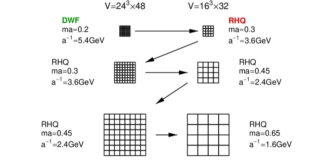
Figure 1: A schematic of the step scaling technique we use to determine the $m$, $c_{B}$,$c_{E}$ and $\zeta$, appropriate for charm quark physics, from non-perturbative, $O(a)$-improved, light quark calculations at $1/a=5.4$ GeV.

Figure 1 shows the steps that we have begun to carry out. Using the quenched approximation for simplicity, we match physical quantities calculated on the two finest lattices, which have a fixed physical volume of $(0.9fm)^{3}$. For the $1/a=5.4$ GeV lattice we use domain wall fermions (DWF), involving the single parameter, $m\approx 1.08$ GeV, chosen to approximate the charm quark mass. We then adjust the coefficients of the RHQ action on the $1/a=3.6$ lattice until the spectra of the two calculations agree. Second, we expand the volume to $(1.35fm)^{3}$, keeping all coefficients fixed, and then match with a fourth calculation with 3/2 larger lattice spacing. Here, we demonstrate the practical implementation of our approach through stage one: matching the DWF 5.4 GeV (fine lattice) spectrum calculated that on a 3.6 GeV (coarse lattice) using the RHQ action.

In the matching step we compare the pseudo-scalar(PS), vector(V), scalar(S), and pseudo-vector(PV) meson masses for heavy-heavy(hh) states and PS and V masses for heavy-light(hl) states. We also require the equality of the masses $m_{1}$ and $m_{2}$ in the hh-PS dispersion relation $E(p^{2})^{hh}_{PS}=m_{1}^{2}+(m_{1}/m_{2})p^{2}$. For both the heavy quark on the fine lattice and the light quark at both lattice spacings we use the DWF action, see Ref. [Blum:2000kn] for the method used here and further references. In each case we used a fifth dimensional extent, $L_{s}=12$ and a domain wall “height”, $M_{5}=1.5$, ensuring that there are no unphysical propagating states for the quark masses used.

As a starting point for our $1/a=3.6$ GeV calculation, we used the one-loop perturbative coefficients for the five-parameter Tsukuba action [Aoki:2003dg]. These were translated into the four parameters of the Fermilab RHQ action by performing the $O(a)$ tree-level field transformation:

$$\psi_{T}=[1+\delta\vec{\gamma}\vec{D}]\psi_{F},\quad\overline{\psi}_{T}=\overline{\psi}_{F}[1-\delta\vec{\gamma}\stackrel{{\scriptstyle\leftarrow}}{{D}}],\quad\delta=\frac{-r_{s}-\zeta}{2(m_{0}+\zeta)}.$$ (5)

3 Simulation

We used the Wilson gauge action since its relation between coupling and lattice spacing has been carefully studied [Necco:2001xg]. However, as a final check, we examined the static quark potential on our two ensembles. We first determined the lattice spacing directly from the two standards scales, $r_{0}$ and $r_{I}$, obtaining results distorted by our small-volumes. We also obtained the ratio of lattice spacings directly from the following relation:

$$V_{1}(n_{1})=V_{2}(n_{2}/\lambda)/\lambda+C$$ (6)

where $\lambda(={a_{2}}/{a_{1}})$ is the lattice spacing ratio between two lattices. The potential $V_{2}(r)$, from the fine lattice, is fit to a standard phenomenological form and then $\lambda$ determined so that this fit, scaled as in Eq. 6 matches that on the coarse lattice, giving the expected ratio $a_{1}/a_{2}=1.51(2)$. Figure. 2 shows how accurately these scaled static quark potentials agreed.

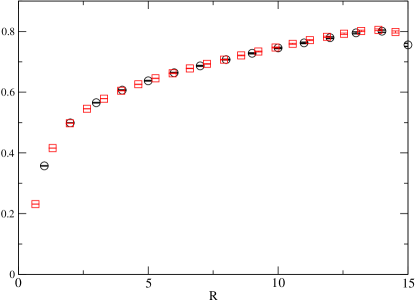
Figure 2: The squares are the static quark potential from the $\beta$ = 6.638 lattice scaled to match the lattice spacing at $\beta$ = 6.351. The circles are the $\beta$ = 6.351 potential.

We employed a “smeared”, Coulomb gauge-fixed, heavy quark wavefunction source using orthogonal hydrogen ground and first-excited wavefunctions. Table 1 lists the 22 RHQ parameter sets that we have run on the coarse lattices. The first few sets of data were chosen close to the 1-loop coefficients described above and the latter ones adjusted as we further explored the parameter space.

Table 1: The details of the parameters we have run for the work reported here.

Label	$m_{0}$	$c_{B}$	$c_{E}$	$\zeta$
1	0.00	1.552	1.458	1.013
2	0.07	1.547	1.424	1.001
3	0.0426	1.550	1.438	1.007
4	0.0426	1.550	1.438	1.100
5	0.0426	1.550	1.438	0.900
6	0.0330	1.609	1.538	1.044
7	0.0230	1.609	1.438	1.044
8	0.0230	1.609	1.538	1.044
9	0.0426	1.609	1.438	1.044
10	0.0426	1.550	1.438	1.007
11	0.0	1.552	1.438	1.013

Label	$m_{0}$	$c_{B}$	$c_{E}$	$\zeta$
12	0.0328	1.511	1.438	1.036
13	0.0230	1.511	1.438	1.036
14	0.0328	1.511	1.538	1.036
15	-0.01	1.700	1.574	1.022
16	0.00371	1.709	1.577	1.023
17	0.0138	1.715	1.579	1.025
18	0.02	1.719	1.580	1.026
19	0.03	1.725	1.582	1.027
20	0.08	1.707	1.576	1.023
21	0.09	1.713	1.578	1.025
22	0.1	1.719	1.580	1.026

4 Analysis and result

We next use the above parameter sets to determine the dependence of the measured quantities on the four RHQ action parameters we wish to determine. We attempt to work within a parameter range where we can use the linear relation:

$$Y_{coarse}^{i}=A+J\cdot X_{RHQ}^{i}$$ (7)

Here $A$ is a $d$-dimensional vector and $J$ an $d\times 4$ matrix. The vector $X_{RHQ}^{i}$ is formed of the four RHQ parameters $\{(X_{RHQ})_{a}^{i}\}_{1\leq a\leq 4}=\{m_{0}^{i},c_{B}^{i},c_{E}^{i},\zeta^{i}\}$ while the $d$-dimensional vector $Y_{coarse}^{i}$ is formed from the spectral quantities measured on the coarse lattice. For $d=6$ $\{(Y_{coarse}^{i})_{a}\}_{1\leq a\leq 6}=\{\frac{1}{4}(M_{PS}+3M_{V})^{hh,i},(M_{PS}-M_{V})^{hh,i},(M_{PV}-M_{S})^{hh,i},(m_{1}/m_{2})^{hh,i},\frac{1}{4}(M_{PS}+3M_{V})^{hl,i},(M_{PS}-M_{V})^{hh,i}\}$. The index $i$ labels the parameter set and varies between 1 and 22.

Equation 7 can be solved directly for $A$ and $J$ if we use five parameter sets. More parameter sets can be used if we minimize a weighted sum of the deviations between the left- and right-hand sides of Eq. 7. We can then use the resulting values for $J$ and $A$, to solve for the parameters $X_{RHQ}$ that yield meson masses as close as possible to those on the fine lattice (denoted as $Y_{fine}$ with error $\sigma_{fine}$) by minimizing the following quantity with respect to $X_{RHQ}$:

$$\chi_{fine}^{2}=\sum_{n=1}^{d}\frac{|(J\cdot X_{RHQ}+A-Y_{fine})_{n}|^{2}}{\sigma_{fine,n}^{2}}.$$ (8)

We divided our data into three categories to explore the sensitivity of the resulting coefficients to our choice of masses being matched: A. heavy-heavy system only, including spin-orbit splitting; B. heavy-heavy (no SO splitting) and heavy-light systems; and C. all of the above measurements. The first five rows of Table 2 demonstrate the stability of our results for the least constrained choice of set A. As we incrementally removed the parameter sets that contribute the most to the chi-squared in Eq. 8, the matching RHQ parameters remain consistent.

Table 2: A check on the stability of the analysis using the example of data set A and results for B and C. Note, the errors on $m_{0}$ should be viewed as  20% of the $\approx 0.3$ renormalized mass.

data sets	$\chi^{2}/d.o.f.$	$m_{0}$	$c_{B}$	$c_{E}$	$\zeta$
A(all)	512/22	0.035(61)	1.725(10)	1.3(5)	1.036(17)
(drop 15)	123/21	0.034(60)	1.726(10)	1.3(5)	1.036(17)
(drop 4,15)	57/20	0.027(66)	1.71(9)	1.3(4)	1.039(18)
(drop 3, 4, 15)	41/19	0.026(67)	1.71(9)	1.3(4)	1.039(18)
(drop 2, 3, 4, 15)	29/18	0.026(65)	1.70(9)	1.3(4)	1.040(18)
B	128/21	0.03(21)	1.75(18)	1.3(17)	1.04(4)
C	42/19	0.011(61)	1.73(1)	1.2(4)	1.043(17)

As Table 2 suggests, we have very consistent results for different choices of parameter sets and meson masses to be matched. The results from parameter set B, which excludes the spin-orbit splitting, gives $c_{E}$ and $m_{0}$ with enormous errors. On the other hand, the matching coefficients determined from sets A and C look more promising.

5 Outlook and Conclusion

It appears practical to determine $m_{0}$, $c_{B}$, $c_{E}$ and $\zeta$ from finite-volume, non-perturbative matching. More statistics and better parameter coverage should reduce the matching errors to a few percent. Carrying out the second matching step in Fig. 1 will permit us to perform a RHQ, charm physics calculation with $1/a=2.4$ GeV and a $(2{\rm fm})^{3}$ volume. While we have reported quenched results here, it should be emphasized that this approach can be extended to full QCD without excessive computational cost. Since the RHQ parameters being determined are short-distance quantities, they depend on both the lattice volume and sea quark masses only through $O(a^{2})$ errors. Hence the dynamical quark masses need not be physical but must only obey $m_{\rm sea}\ll 1/a$. Thus, we need only require that $N_{f}=3$ and that $m_{sea}$/$\Lambda_{QCD}$ are equal for each pair of systems being matched.