Spectral properties of the Landau gauge Faddeev-Popov operator in lattice gluodynamics

Abstract

Recently we reported on the infrared behavior of the Landau gauge gluon and ghost dressing functions in $SU(3)$ Wilson lattice gluodynamics with special emphasis on the Gribov problem. Here we add an investigation of the spectral properties of the Faddeev-Popov operator at $\beta=5.8$ and $6.2$ for lattice sizes $12^{4}$, $16^{4}$ and $24^{4}$. The larger the volume the more of its eigenvalues are found accumulated close to zero. Using the eigenmodes for the spectral representation it turns out that for our smallest lattice $\mathcal{O}(200)$ eigenmodes are sufficient to saturate the ghost propagator at lowest momentum. We associate exceptionally large values of the ghost propagator to extraordinary contributions of low-lying eigenmodes.

I Introduction

The infrared suppression of the gluon propagator on the one hand and the enhancement of the ghost propagator at low momentum on the other are closely related to the Gribov-Zwanziger horizon condition Zwanziger (2004, 1994); Gribov (1978) as well as to the Kugo-Ojima confinement criterion Kugo and Ojima (1979). Zwanziger Zwanziger (2004) has worked out that the continuum behavior of both propagators in Landau gauge are consequences of restricting gauge fields to the Gribov region $\Omega$, where the Faddeev-Popov operator is non-negative. In general, for a given gauge field a gauge orbit has more than one intersection (Gribov copy) within $\Omega$. However, in the infinite volume limit expectation values taken over arbitrary representatives of $\Omega$ are predicted to be equal to those over the fundamental modular region $\Lambda$, the set of gauge fields being absolute maxima of the Landau gauge functional defined below. On a finite lattice, however, this equality cannot be expected Zwanziger (2004). Therefore, the Gribov ambiguity has to be explored in detail on finite lattices before drawing any conclusion about the infrared behavior of the propagators mentioned. In previous investigations Cucchieri (1997); Bakeev et al. (2004); Sternbeck et al. (2005) the influence of Gribov copies on the Landau gauge ghost and gluon propagators was studied in detail both for $SU(2)$ and $SU(3)$. Whereas the gluon propagator was not seen to be influenced by the choice of gauge copies the ghost propagator turned out to be clearly copy-dependent in the limit of small momenta.

In the present letter we are asking, how the singular behavior of the ghost propagator is related to the spectrum of the Landau gauge Faddeev-Popov (F-P) operator. It is exactly there that the Gribov ambiguity must become visible. We will demonstrate that the low-lying eigenvalues move towards zero as the volume increases and that their values are sensitive to the choice of Gribov copies. We will also discuss the localization properties of the corresponding eigenmodes. The mode expansion of the momentum space ghost propagator will be shown to converge the slower the higher the momentum is. Returning to the problem of exceptionally large values of the ghost propagator (“exceptional configurations”), discussed in Bakeev et al. (2004); Sternbeck et al. (2005), we can show that they are related to strong contributions of the lowest eigenmodes. For the sake of completeness we remind of a recent investigation of the spectrum of the Coulomb gauge F-P operator Greensite et al. (2005).

We introduce relevant definitions and notations in Sec. II. Simulation details are given in Sec. III. In Sec. IV the spectral properties of the F-P operator are discussed. Configurations with exceptionally large values for the ghost propagator are studied in Section V. In Section VI we will draw our conclusions.

II Definitions

In order to study the ghost propagator using lattice simulations one has to fix the gauge for each thermalized $SU(3)$ gauge field configuration $U\equiv\{U_{x,\mu}\}$. We apply the Landau gauge condition which can be implemented as a search for a gauge transformation $g\equiv\{g_{x}\}$

$$U_{x,\mu}\rightarrow{}^{g}U_{x,\mu}=g_{x}\,U_{x,\mu}\,g^{\dagger}_{x+\hat{\mu}}\,,\quad g_{x}\in SU(3)$$

that maximizes the Landau gauge functional

$$F_{U}[g]=\frac{1}{4V}\sum_{x}\sum_{\mu=1}^{4}\mathfrak{Re}\,\mbox{Tr}\;{}^{g}U_{x,\mu}$$ (1)

while keeping the link variables $U_{x,\mu}$ fixed.

The functional $F_{U}[g]$ has many different local maxima. When the lattice volume $V$ is enlarged for a fixed inverse coupling constant $\beta$ or, alternatively, $\beta$ is decreased, more and more of these maxima become accessible by an iterative gauge fixing process starting from various initial random gauge transformations. The set of gauge copies $\{{}^{g}U\}$ which correspond to different (local) maxima of $F_{U}[g]$, where $U$ is kept fixed, are called Gribov copies in analogy to the Gribov ambiguity in the continuum Gribov (1978). All Gribov copies belong to the gauge orbit created by $U$ and satisfy the differential (lattice) Landau gauge transversality condition $(\partial_{\mu}{}^{g}\!\!A_{\mu})(x)=0$ where

$$(\partial_{\mu}{}^{g}\!\!A_{\mu})(x)\equiv\sum_{\mu}\left({}^{g}\!\!A_{\mu}(x+\hat{\mu}/2)-{}^{g}\!\!A_{\mu}(x-\hat{\mu}/2)\right)\,.$$ (2)

Here ${}^{g}\!\!A_{\mu}(x+\hat{\mu}/2)$ defines the non-Abelian gauge potential on the lattice, i.e.

$${}^{g}\!\!A_{\mu}(x+\hat{\mu}/2)\equiv\frac{1}{2i}\left({}^{g}U_{x,\mu}-\ ^{g}U^{\dagger}_{x,\mu}\right)\Big{|}_{\rm traceless}\,.$$ (3)

In the following, we will drop the label $g$ for convenience, i.e. we assume $U$ to satisfy the Landau gauge condition such that $g\equiv\mathbb{1}$ maximizes the functional in Eq. (1) relative to the neighborhood of the identity.

The F-P operator is the Hessian of the gauge functional Eq. (1) and can be expressed in terms of the (gauge-fixed) link variables $U_{x,\mu}$ as

$$M^{ab}_{xy} = \sum_{\mu}A^{ab}_{x,\mu}~{}\delta_{x,y}-B^{ab}_{x,\mu}~{}\delta_{x+\hat{\mu},y}-C^{ab}_{x,\mu}~{}\delta_{x-\hat{\mu},y}\quad$$ (4)

$$\textrm{with}\quad A^{ab}_{x,\mu} = \phantom{2\cdot\ }\mathfrak{Re}\,\mbox{Tr}\left[\{T^{a},T^{b}\}(U_{x,\mu}+U_{x-\hat{\mu},\mu})\right],$$

$$B^{ab}_{x,\mu} = 2\cdot\mathfrak{Re}\,\mbox{Tr}\left[T^{b}T^{a}\,U_{x,\mu}\right],$$

$$C^{ab}_{x,\mu} = 2\cdot\mathfrak{Re}\,\mbox{Tr}\left[T^{a}T^{b}\,U_{x-\hat{\mu},\mu}\right]\;.$$

Here $T^{a}$ ($a=1,\ldots,8$) denote the generators of the $\mathfrak{su}(3)$ Lie algebra satisfying $\mbox{Tr}[T^{a}T^{b}]=\delta^{ab}/2$.

For each maximum of the gauge functional $F_{U}[g]$ the corresponding F-P operator has only positive eigenvalues $\lambda_{i}>0$, $(i=1,\ldots,8V-8)$, besides of its eight trivial zero modes, i.e. the gauge-fixed field configurations $U$ lie within the Gribov region $\Omega$. We expect that the spectral properties of the F-P operator differ for different Gribov copies. This should have consequences for the ghost propagator. We will exploit the spectral representation of the inverse of the F-P operator for a given gauge field $U$ in terms of its real (ascendent) eigenvalues $\lambda_{i}$ and its (normalized) eigenvectors $\vec{\phi}_{i}(x)$ in coordinate space

$$[M^{-1}(U)]^{ab}_{xy}=\sum_{i=1}^{N}\phi_{i}^{a}(x)\frac{1}{\lambda_{i}}\phi_{i}^{b}(y)\;.$$ (5)

The eigenvectors are given at each lattice point $x$ as $8$-component color vectors $\vec{\phi}_{i}$ with components $\phi^{a}_{i}(x)$. They are normalized such that $\sum_{x}|\vec{\phi}_{i}(x)|^{2}=1$. Taking their Fourier transformed vectors $\vec{\Phi}_{i}(k)$ for momenta $k_{\mu}\in(-L_{\mu}/2,+L_{\mu}/2]$ and averaging over a Monte Carlo (MC) generated ensemble of gauge field configurations we have computed the ghost propagator from truncated mode expansions

$$G_{n}(q)=\langle G(k|n)\rangle_{\textrm{MC}}$$ (6)

where

$$G(k|n)=\frac{1}{8}~{}\sum_{i=1}^{n}\frac{1}{\lambda_{i}}\,\vec{\Phi}_{i}(k)\cdot\vec{\Phi}_{i}(-k)$$ (7)

denotes the contribution of the eigenvalues and eigenmodes on a given gauge field configuration. Here the vector and scalar product notation refers to the color indices. The Fourier momenta $k_{\mu}$ are related to the physical momenta $q_{\mu}$ by

$$q_{\mu}(k_{\mu})=(2/a)\sin(\pi k_{\mu}/L_{\mu})$$

with $a$ and $L_{\mu}$ denoting the lattice spacing and the linear lattice extension, respectively.

If for the whole ensemble of configurations all $N=8(V-1)$ non-trivial eigenvalues and eigenvectors were known, the ghost propagator would be determined completely, i.e. $G(q)\equiv G_{N}(q)$ at all momenta. We will check the convergence with respect to the order $n$ by comparing the truncated propagator $G_{n}(q)$ with the full one, $G(q)$, obtained by inverting $M$ for a set of plane wave sources (with $\vec{k}\neq 0$) orthogonal to the trivial zero-modes. For details we refer to reference Sternbeck et al. (2005).

From Eq. (7) it is evident that the low-lying eigenvalues and eigenvectors have a dominating impact on the ghost propagator. However, for a finite lattice size it is not a priori obvious what fraction of the F-P spectrum is responsible for the enhancement of the ghost propagator at the smallest available momenta. Zwanziger has argued that the F-P operator has very small eigenvalues Zwanziger (2004). In particular, it should have a high density $\rho(\lambda)$ of eigenvalues per unit Euclicean volume at the Gribov horizon (for $\lambda>0$). This causes the ghost propagator to diverge stronger than $1/q^{2}$ at $q=0$ Zwanziger (2004). We estimate the eigenvalue density $\rho$ at small $\lambda$ by

$$\rho(\lambda)=\frac{h(\lambda,\lambda+\Delta\lambda)}{N\Delta\lambda}\,,$$ (8)

the average number $h$ of eigenvalues per gauge-fixed configuration within the interval $[\lambda,\lambda+\Delta\lambda]$ divided by the bin size $\Delta\lambda$. For normalization the denominator $N=8V$ has been chosen, since the F-P matrix is a $N\times N$ sparse symmetric matrix with $N$ linearly independent eigenstates. Note, the trivial zero modes are described by a $8\delta(\lambda)$-peak at $\lambda=0$.

III Simulation details

For the purpose of this study we have analyzed pure $SU(3)$ gauge configurations thermalized with the standard Wilson action at two values of the inverse coupling constant $\beta=5.8$ and $6.2$. Cycles of one heatbath and four micro-canonical over-relaxation steps were used for thermalization. As lattice sizes we used $12^{4}$, $16^{4}$ and $24^{4}$. To each thermalized configuration $U$ a set of $N_{\rm cp}{}$ random gauge transformations was assigned. Each has served as a starting point for a gauge fixing procedure. We have applied standard over-relaxation with over-relaxation parameter tuned to $w=1.63$. Keeping $U$ fixed this iterative procedure generates a sequence of gauge transformations with increasing values of the gauge functional (Eq. (1)). Thus, the final Landau gauge is iteratively approached until the stopping criterion in terms of the transversality (see Eq. (2))

$$\max_{x}\mbox{Tr}\left[\partial_{\mu}{}^{g}\!\!A_{\mu}(x)\partial_{\mu}{}^{g}\!\!A^{\dagger}_{\mu}(x)\right]<10^{-14}$$ (9)

was fulfilled. Consequently, each random start leads to its own local maximum of the gauge functional. However, certain extrema of the functional are found multiple times. This happened frequently for the $12^{4}$ lattices, but rather seldom on larger ones. Note, we used the worst local violation of transversality as stopping criteria which at a first glance seems to be very conservative. However, we have found that the precision of transversality is crucial for the final precision of the ghost propagator at low momentum.

In order to study the dependence on Gribov copies, for each $U$ that copy with largest functional value — among all $N_{\rm cp}{}$ gauge-fixed ones — was stored, labeled as best copy (bc). The larger $N_{\rm cp}{}$, the bigger the likeliness that this copy represents the absolute maximum of the functional in Eq. (1), at least with respect to the observable in question. Indeed, with an increasing number $N_{\rm cp}{}$ of inspected gauge copies for each $U$, the expectation values of the ghost and gluon propagator evaluated on bc copies is found to converge more or less rapidly Sternbeck et al. (2005). The first gauge copy was also stored, labeled as first copy (fc). Obviously, this copy is as good as any other arbitrarily selected one.

On those ensembles of fc and bc gauge-fixed configurations the low-lying eigenvalues $\lambda$ of the F-P operator and the corresponding eigenmodes have been separately extracted, where we used the parallelized version of the ARPACK package Rich Lehoucq et al. , PARPACK. To be specific, the 200 lowest (non-trival) eigenvalues and their corresponding eigenfunctions have been calculated at $\beta=6.2$ using the lattice sizes $12^{4}$ and $16^{4}$ (see Table 1). On the $24^{4}$ lattice, due to restricted amount of computing time, only 50 eigenvalues and eigenmodes have been extracted at the same $\beta$. In addition, 90 eigenvalues have been calculated on a $24^{4}$ lattice at $\beta=5.8$ providing us with an even larger physical volume. This allows us to check whether low-lying eigenvalues are shifted towards $\lambda\to 0$ as the physical volume is increased.

No.	$\beta$	lattice	# conf	# copies	# eigenvalues
1	6.2	$12^{4}$	150	20	200
2	6.2	$16^{4}$	100	30	200
3	6.2	$24^{4}$	35	30	50
4	5.8	$24^{4}$	25	40	90

Table 1: Statistics of the data used in our analysis. The last column lists the number of eigenvalues extracted separately on fc and bc copies of $U$. At $\beta=6.2$ the corresponding eigenmodes were calculated, too.

IV The spectral properties of the F-P operator

IV.1 The spectrum of the low-lying eigenvalues

Let us first discuss the distributions of the lowest $\lambda_{1}$ and second lowest $\lambda_{2}$ eigenvalue of the F-P operator. These are shown for different volumes in Fig. 1. There $h(\lambda,\lambda+\Delta)$ refers to the average number (per configuration) of eigenvalues found in the intervall $[\lambda,\lambda+\Delta]$. Open (full) bars refer to the distribution on fc (bc) gauge copies.

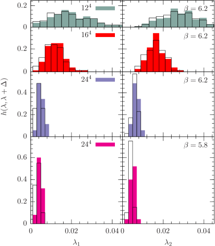
Figure 1: The frequency $h(\lambda)$ per configuration of the lowest (left panels) and second lowest (right panels) eigenvalue $\lambda$ of the Faddeev-Popov operator is shown. Filled boxes represent the distribution obtained on bc gauge copies, while open ones represent those on fc copies.

From Fig. 1 it is quite obvious that both eigenvalues $\lambda_{1}$ and $\lambda_{2}$ are shifted to lower values as the physical volume is increased. In conjunction the spread of $\lambda$ values is decreased. This would be even more obvious, if we had shown both distributions as functions of $\lambda$ in physical units. It is also visible that the two low-lying eigenvalues $\lambda^{\texttt{fc}}_{i}$ ($i=1,2$) on fc gauge copies tend to be lower than those on bc copies. However, this holds only on average as can be seen from Fig. 2. There the differences $\lambda^{\texttt{bc}}_{1}-\lambda^{\texttt{fc}}_{1}$ of the lowest eigenvalues on fc and bc gauge copies are shown for different lattice sizes at $\beta=6.2$ and $5.8$. It is quite evident that there are few cases where $\lambda^{\texttt{bc}}_{1}<\lambda^{\texttt{fc}}_{1}$, even though $F^{\texttt{bc}}\geq F^{\texttt{fc}}$ always holds for the gauge functional.

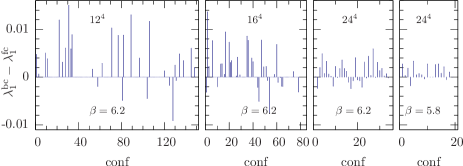
Figure 2: The differences $\lambda^{\texttt{bc}}_{1}-\lambda^{\texttt{fc}}_{1}$ of the lowest F-P eigenvalues calculated on bc and fc representatives for each gauge configuration are shown. From left to right the lattice sizes are $12^{4}$, $16^{4}$ and $24^{4}$ at $\beta=6.2$ and $24^{4}$ at $\beta=5.8$.

In addition we have checked how the average values $\langle\lambda\rangle$ of the eigenvalue distributions tends towards zero as the linear extension $aL$ of the physical volume is increased. As in our previous study Sternbeck et al. (2005) we followed Ref. Necco and Sommer (2002) to fix the lattice spacing $a$. For $\beta=5.8$ and 6.2 we used $a^{-1}$=1.446 GeV and 2.914 GeV, respectively, using the Sommer scale $r_{0}=0.5$ fm.

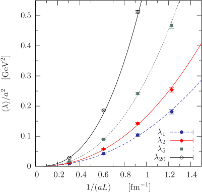
Figure 3: The average values $\langle\lambda_{i}\rangle/a^{2}$ (scaled to physical units) of the eigenvalues $\lambda_{i}$ $(i=1,2,5,20)$ are shown vs. the inverse of the linear lattice extension $aL$. Only eigenvalues on bc copies are shown. The lines represent fits to the data using the ansatz $a^{-2}\langle\lambda_{i}\rangle=C_{i}/(aL)^{2+\epsilon_{i}}$.

If the low-lying eigenvalues are supplemented with physical units it turns out that the average values of their distributions tend towards zero stronger than $1/(aL)^{2}$. In fact, using the ansatz

$$f(aL)=\frac{C}{(aL)^{2+\varepsilon}}$$ (10)

to fit the data of $\langle\lambda_{i}\rangle/a^{2}$ for different $(aL)$, a positive $\varepsilon$ is found. The parameter of these fits are given in Table 2 and in Fig. 3 we show the data and the corresponding fitting functions. There one clearly sees, the low-lying eigenvalues not only approach zero, but also become closer to each other with increasing $aL$. We have addressed the latter issue by fitting the differences $(\langle\lambda_{i+1}\rangle-\langle\lambda_{i}\rangle)/a^{2}$ of adjacent average values using the same ansatz Eq. (10). In Table 2 we give the parameter of those fits.

As mentioned in Sec. II the eigenvalue density $\rho(\lambda)$ is of particular interest. We have estimated this quantity according to Eq. (8) where the bin sizes have been reasonably adjusted for the different volumes. In Fig. 4 the estimates are shown for two values of $\beta$. There one clearly sees the eigenvalue density close to $\lambda=0$ becomes a steeper function of $\lambda$ as the physical volume becomes larger. It is remarkable that the increase going from $\beta=6.2$ to $\beta=5.8$ on a $24^{4}$ lattice is even larger than going from $12^{4}$ to $24^{4}$ at $\beta=6.2$, although in both cases the physical volume is increased by a factor of about 16.

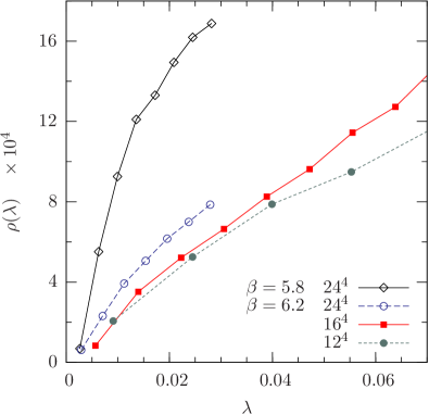
Figure 4: The eigenvalue density $\rho$ for bc copies as a function of $\lambda$ estimated on $12^{4}$ and $16^{4}$ lattices at $\beta=6.2$ and on a $24^{4}$ lattice for $\beta=6.2$ and $5.8$. Bin sizes have been chosen as small as possible for each lattice size. The points marks the middle of each bin and the lines are to guide the eye.

$a^{2}f(aL)$	$C$	$\epsilon$	$\chi^{2}/\textsc{ndf}$
$\langle\lambda_{1}\rangle$	0.120(3)	0.16(4)	0.7
$\langle\lambda_{2}\rangle$	0.165(4)	0.24(5)	1.8
$\langle\lambda_{5}\rangle$	0.290(1)	0.45(4)	3.5
$\langle\lambda_{2}\rangle-\langle\lambda_{1}\rangle$	0.045(2)	0.47(9)	0.4
$\langle\lambda_{3}\rangle-\langle\lambda_{2}\rangle$	0.051(1)	0.88(8)	0.2
$\langle\lambda_{4}\rangle-\langle\lambda_{3}\rangle$	0.033(1)	0.62(33)	2.0
$\langle\lambda_{5}\rangle-\langle\lambda_{4}\rangle$	0.037(1)	0.89(1)	0.003

Table 2: The parameter $C$ and $\epsilon$ from fitting either the averages $\langle\lambda_{i}\rangle/a^{2}$ or the differences of adjacent average values $\langle\lambda_{i+1}\rangle/a^{2}-\langle\lambda_{i}\rangle/a^{2}$ of the corresponding eigenvalue distributions to the ansatz $f(aL)=C_{i}/(aL)^{2+\epsilon_{i}}$.

Figure 5: The relative distribution $h$ of IPR values of the 10 (left), the 10 to 20 (middle) and the 20 to 50 (right) lowest eigenmodes are shown. Note there is a logarithmic scale for $h(\mbox{\tt IPR}{})$. Each row corresponds to one pair of $\beta$ and lattice size. Filled boxes refer to distributions on bc gauge copies, while open ones correspond to fc copies.

IV.2 Localization properties

Together with the low-lying eigenvalues the corresponding eigenvectors $\vec{\phi}(x)$ have been extracted as well. It is interesting to evaluate for each vector the inverse participation ratio (IPR). The IPR is defined as

$$\mbox{\tt IPR}=V\sum_{x}|\vec{\phi}(x)|^{4}\qquad\textrm{with}\;V=L^{4}$$

and is a measure for the localization of an eigenvector. It enables us to distinguish between eigenmodes with approximately uniformly distributed values of $|\vec{\phi}(x)|^{2}$ ($\mbox{\tt IPR}\approx 1\ldots 2$) and specific ones with a small number of sites $x$ having large modulus squared $|\vec{\phi}(x)|^{2}$ ($\mbox{\tt IPR}\sim\rm{O}(100)$). Note, the eight (trivial) zero modes ($\lambda=0$) of the F-P operator give all $\mbox{\tt IPR}{}=1$.

From Fig. 5 we learn that the majority of eigenvectors of the Faddeev-Popov operator is not localized. However, some large IPR values have been found associated with modes among the 10 lowest non-zero eigenmodes. This becomes more likely as the volume is increased. So far we have no physical interpretation what causes the stronger localization in these rare cases.

IV.3 What fraction of the F-P spectrum is dominating the ghost operator?

As we have mentioned in Sec. II there is an obvious way to construct the ghost operator, if all eigenvalues $\lambda_{i}$ of the F-P operator and the corresponding eigenvectors $\vec{\Phi}_{i}(k)$ in momentum space would be available. However, their determination for each configuration is numerically too demanding.

Restricting the sum in Eq. (7) to the $n$ lowest eigenvalues and eigenvectors ($n\ll N=8V-8$), we can figure out to what extent these modes, i.e. the corresponding estimator $G_{n}(q)$ in Eq. (6), saturate the full ghost propagator $G(q)$ obtained independently for a set of momenta by inverting the F-P matrix on plane waves. See our recent study Sternbeck et al. (2005) for the data of $G(q)$.

This saturation is shown in Fig. 6 for the lowest $q_{1}$ and the second lowest momentum $q_{2}$ available on different lattice sizes for $\beta=6.2$. There the values of $G_{n}(q)$ have been divided by the values for the full propagator $G(q)$ in order to compare the saturation for different volumes. Since $\vec{\Phi}_{i}(k)$ has been obtained by a fast Fourier transformation of the eigenvector $\vec{\phi}_{i}(x)$, all lattice momenta $k$ are available. Thus $G_{n}(q)$ refers to the average over all $k$ giving raise to the same momentum $q$. The full propagator values $G(q)$ at $q_{1}(k)$ and $q_{2}(k)$, however, refer to the averages over lattice momenta $k=([1,0],0,0)$ and to $k=(1,1,0,0)$, respectively.

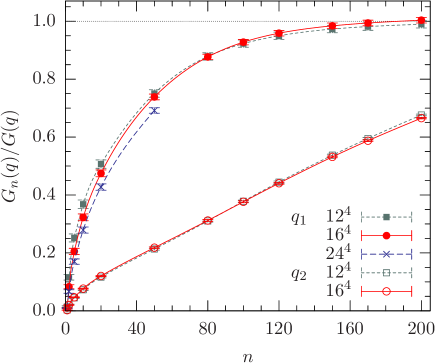
Figure 6: The ratio of the truncated ghost propagator $G_{n}(q)$ (in terms of the $n$ lowest F-P eigenmodes and eigenvalues) to the full estimate $G(q)$ (taken from Sternbeck et al. (2005)) shown as a function of $n$ for the lowest ($q_{1}$) and second lowest ($q_{2}$) momentum. The inverse coupling is $\beta=6.2$ and the lattice size ranges from $12^{4}$ to $24^{4}$. The data refer to bc copies.

Let us consider first the lowest momentum $q_{1}$. We observe from Fig. 6 that the approach to convergence differs, albeit slightly, for the three different lattice sizes. The relative deficit for $n<50$ rises with the lattice volume. For $n>100$ the rate on a $16^{4}$ lattice is even a bit larger than that on a $12^{4}$ lattice. Unfortunately, there are no data available for $n>50$ on the $24^{4}$ lattice. However, for the $12^{4}$ and $16^{4}$ lattices the rates of convergence are about the same. For example, taking only 20 eigenmodes one is definitely far from saturation (by about 50%) whereas $150\ldots 200$ eigenmodes are sufficient to reproduce the ghost propagator within a few percent. In other words, the ghost propagator at lowest momentum on a $12^{4}$ ($16^{4}$) lattice is formed by about 0.12% (0.03%) of the lowest eigenvalues and eigenfunctions of the F-P operator.

For the second lowest momentum $q_{2}$ the contribution of even 200 eigenmodes is far from being sufficient to approximate the propagator.

V The problem of exceptional configurations

We turn now to a peculiarity of the ghost propagator at larger $\beta$ of which we have reported in Sternbeck et al. (2005). It was also seen by two of us in an earlier $SU(2)$ study Bakeev et al. (2004). While inspecting our data we found, though rarely, that there are exceptionally large values in the Monte Carlo (MC) time histories of the ghost propagator at lowest momentum. Those values are not equally distributed around the average value, but rather are significantly larger. For details we refer to reference Sternbeck et al. (2005).

We have tried to find a correlation of such exceptionally large values in the history of the ghost propagator with other quantities measured in our simulations. For example we have checked whether there is a direct correlation between the values of the ghost propagator $G(k)$ as they appear in the MC time histories (see e.g. Fig. 5 in Sternbeck et al. (2005)) and the lowest eigenvalue $\lambda_{1}$ of the F-P operator.

In Fig. 7 we show such correlation in a scatter plot for different lattice sizes at $\beta=5.8$ and $6.2$. There each entry corresponds to a pair $[\lambda_{1},G(k)]$ measured on a given gauge copy of our sets of fc and bc copies. It is visible in that figure, gauge copies giving rise to an extremely large MC value for the ghost propagator are those with very low values for $\lambda_{1}$. This holds for the $12^{4}$ and $16^{4}$ lattice. However, a very low eigenvalue is not sufficient to obtain large MC values for $G(k)$ as can be seen in the same figure. It is not excluded that such gauge copies with extremely small eigenvalues would turn out to be exceptional for another realization of lowest momentum $q(k)$ than those two we have used. This might explain why some configurations with extremely small lowest eigenvalues were not found to be exceptional with respect to the ghost propagator at $k=(1,0,0,0)$ and $k=(0,1,0,0)$.

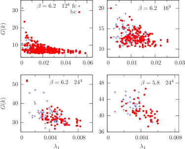
Figure 7: Scatter plots of MC time history values of the ghost propagator $G(k)$ at $k=([1,0],0,0)$ vs. the lowest F-P eigenvalue $\lambda_{1}$ are shown. The upper panels show data at $\beta=6.2$ on a $12^{4}$ (left) and $16^{4}$ (right) lattice, the lower ones on a $24^{4}$ lattice at $\beta=6.2$ (left) and $\beta=5.8$ (right). Crosses refer to fc gauge copies and filled circles to bc copies.

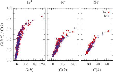
Figure 8: Scatter plot of the relative contribution of the truncated sums $G(k|n)$ over eigenmodes (see Eq. (7)) to the full ghost propagator values $G(k)$ versus $G(k)$ for lattice momenta $k=(1,0,0,0)$ and $k=(0,1,0,0)$. From left to right the lattice sizes are $12^{4}$, $16^{4}$ and $24^{4}$ all for $\beta=6.2$. Data for fc and bc gauge copies have been plotted separately.

In the light of Eq. (7) it is not adequate to concentrate just on the lowest eigenvalues. Instead, one can monitor the contribution of a certain number of eigenvalues $\lambda_{i}$ and eigenmodes $\vec{\Phi}_{i}(k)$ to the ghost propagator at some momentum in question. Therefore, we have compared the truncated sums $G(k|n)$ according to Eq. (7) with the MC history values of the full ghost propagator $G$. In fact, we show in the scatter plots in Fig. 8 the ratios $G(k|n)/G(k)$ versus $G(k)$ for $n=10$ and for various lattice sizes.

Obviously there is a strong correlation between the chosen group of low-lying modes and the MC time history values of the full ghost propagator. Indeed, if we consider values $G(k)>15$ to be exceptional in the left-most panel ($12^{4}$ lattice) we find that the contribution of the 10 lowest modes amounts to more than 75% of the actual value of the ghost propagator. On the opposite, for low $G(k)$ values the main contributions come necessarily from the higher eigenmodes, while the 10 lowest modes contribute a minor part only. A similar but less dominant contribution of the 10 lowest modes is found for the time histories produced on larger lattices ($16^{4},~{}24^{4}$).

VI Conclusions

In this paper we have investigated the spectral properties of the F-P operator and their relation to the ghost propagator in $SU(3)$ Landau gauge. The configurations under examination have been generated on a $24^{4}$ lattice at $\beta=5.8$ and on $12^{4}$, $16^{4}$ and $24^{4}$ lattices at $\beta=6.2$.

As expected from Ref. Zwanziger (2004) we have found that the low-lying eigenvalues are shifted towards $\lambda=0$ as the volume is increased. The result is an eigenvalue density $\rho(\lambda)$ becoming steeper rising close to $\lambda=0$. We have also shown that the Gribov ambiguity is reflected in the low-lying eigenvalue spectrum. In fact, the low-lying eigenvalues extracted on bc gauge copies are larger on average than those on fc copies. Thus better gauge-fixing (in terms of the gauge functional) inhibits the above-mentioned tendency, keeping the gauge-fixed configuration slightly away from the Gribov horizon.

The study of the ghost propagator in terms of the eigenvalues and eigenmodes of the F-P operator reveals that there is a dominance of the low-lying part of the spectrum at lowest momentum. About 200 eigenmodes are sufficient to reconstruct the asymptotic result up to a few percent at the lowest momentum on a $12^{4}$ lattice at $\beta=6.2$. With respect to the whole set of $8(12^{4}-1)$ non-trivial eigenvalues, this is a fraction of about 0.12%. For larger volumes the number of necessary eigenmodes seems to be somewhat larger. For the next higher momentum, saturation needs a much bigger part of the low-lying spectrum.

On average the F-P eigenmodes are not localized, however, few large values have been seen among the lowest eigenmodes which so far could not be correlated to other measured quantities.

Analogously with observations made in Ref. Bakeev et al. (2004) we have reported recently Sternbeck et al. (2005) on exceptionally large values in the Monte Carlo history of the ghost propagator. These we have seen at $\beta=6.2$ and only for some lattice momenta $k$ realizing the lowest physical momentum $q(k)$. In the study at hand we have shown that these outliers can be assigned to the contribution of the ten lowest F-P eigenmodes to the ghost propagator at this particular $k$.

References

- Zwanziger (2004) D. Zwanziger, Phys. Rev. D69, 016002 (2004), eprint hep-ph/0303028.
- Zwanziger (1994) D. Zwanziger, Nucl. Phys. B412, 657 (1994).
- Gribov (1978) V. N. Gribov, Nucl. Phys. B139, 1 (1978).
- Kugo and Ojima (1979) T. Kugo and I. Ojima, Prog. Theor. Phys. Suppl. 66, 1 (1979).
- Sternbeck et al. (2005) A. Sternbeck, E.-M. Ilgenfritz, M. Müller-Preussker, and A. Schiller, Phys. Rev. D72, 014507 (2005), eprint hep-lat/0506007.
- Bakeev et al. (2004) T. D. Bakeev, E.-M. Ilgenfritz, V. K. Mitrjushkin, and M. Müller-Preussker, Phys. Rev. D69, 074507 (2004), eprint hep-lat/0311041.
- Cucchieri (1997) A. Cucchieri, Nucl. Phys. B508, 353 (1997), eprint hep-lat/9705005.
- Greensite et al. (2005) J. Greensite, S. Olejnik, and D. Zwanziger, JHEP 05, 070 (2005), eprint hep-lat/0407032.
- (9) R. Rich Lehoucq, K. Maschhoff, D. Sorensen, and C. Yang, Arpack software, URL http://www.caam.rice.edu/software/ARPACK/.
- Necco and Sommer (2002) S. Necco and R. Sommer, Nucl. Phys. B622, 328 (2002), eprint hep-lat/0108008.