HU-EP-05/67

SFB/CPP-05-71

Cutoff effects of Wilson fermions in the absence of spontaneous chiral symmetry breaking

Michele Della Morte^a and Magdalena Luz^a
a Institut für Physik, Humboldt Universität,

Newtonstr. 15, 12489 Berlin, Germany
Abstract

We simulate two dimensional QED with two degenerate Wilson fermions and plaquette gauge action. As a consequence of the Mermin-Wagner theorem, in the continuum limit chiral symmetry is realized à la Wigner. This property affects also the size of the cutoff effects. That can be understood in view of the fact that the leading lattice artifacts are described, in the continuum Symanzik effective theory, by chirality breaking terms. In particular, vacuum expectation values of non-chirality-breaking operators are expected to be O($a$) improved in the chiral limit. We provide a numerical confirmation of this expectation by performing a scaling test.
Key words: Lattice field theory; Schwinger model

PACS: 11.10.Kk; 11.15.-q; 11.15.Ha

October 2005

1. Cutoff effects in lattice (gauge) theories can be described using an effective continuum action, as proposed by Symanzik in refs. [?,?]. In this approach the leading lattice artifacts (e.g. in the spectrum of the theory) can be removed by including a set of irrelevant operators in the action and by properly tuning their coefficients. For the case of the Wilson lattice regularization of QCD [?], the relevant coefficient can be tuned by requiring the restoration of chiral symmetry up to O($a^{2}$). This interplay between chiral symmetry and cutoff effects has been addressed in detail in ref. [?].

Further insights on this connection have been recently derived in ref. [?] by considering also so called spurionic lattice symmetries to classify the operators, which can appear in the Symanzik effective theory. Without reproducing the whole argument, here we will simply summarize the results relevant as premises for this work. Let’s consider the Wilson fermionic action for two degenerate flavors

$$S_{\rm F}[U,\overline{\psi},\psi]=a^{4}\sum_{x}\overline{\psi}(x)(D+m_{0})\psi(x)\quad{\rm and}\;$$ (1)

$$D=\hbox{$1\over 2$}\left\{\gamma_{\mu}(\nabla^{*}_{\mu}+\nabla_{\mu})-ar\nabla^{*}_{\mu}\nabla_{\mu}\right\}\,,$$ (2)

where $\nabla^{*}_{\mu}$ and $\nabla_{\mu}$ are the covariant backward and forward lattice derivative respectively, $U$ denotes the gauge field and $r$ is the Wilson parameter, which we set to 1. The vacuum expectation value of a multiplicatively renormalizable operator $\cal{O}$ can be expanded as

$$\langle\mathcal{O}\rangle|_{r,m_{\rm q}}=\left[\zeta^{\mathcal{O}}+am_{\rm q}\xi^{\mathcal{O}}\right]\langle\mathcal{O}\rangle|^{\rm cont}_{m_{\rm q}}+a\sum\limits_{l}(m_{\rm q})^{n_{l}}\eta^{\mathcal{O}}_{\mathcal{O}_{l}}\langle\mathcal{O}_{l}\rangle|^{\rm cont}_{m_{\rm q}}+{\rm O}(a^{2})\;,$$ (3)

where $m_{\rm q}$ is the bare subtracted fermion mass defined as $m_{\rm q}=m_{0}-m_{\rm c}$, such that the physical fermion mass vanishes for $m_{0}=m_{\rm c}$. We refer to [?] for any unexplained notation in eq. (3). The operators $\mathcal{O}_{l}$ appearing on the rhs result from the insertion of the O($a$) terms in the action and from the O($a$) terms associated with the operator $\mathcal{O}$ itself. They can be classified according to their parity $P_{R_{5}}^{\mathcal{O}_{l}}$ under the $R_{5}$ transformation

$$R_{5}\;:\;\psi\rightarrow\psi^{\prime}=\gamma_{5}\psi\;,\qquad\overline{\psi}\rightarrow\overline{\psi}^{\prime}=-\overline{\psi}\gamma_{5}\;,$$ (4)

which is a non-anomalous element of the chiral group and produces a spurionic symmetry of the Wilson action when combined with the replacements $r\rightarrow-r$, $m_{\rm q}\rightarrow-m_{\rm q}$. The authors of ref. [?] have shown that

$$P_{R_{5}}^{\mathcal{O}}+P_{R_{5}}^{\mathcal{O}_{l}}+n_{l}=1\;{\rm mod}\;(2),$$ (5)

which, loosely speaking, implies that the O($a$) terms in the chiral limit (where the sum reduces to the $n_{l}=0$ contributions) have opposite $R_{5}$-parity compared to the leading term. It is indeed interesting to consider the limit $m_{\rm q}\to 0$ in eq. (3). Two different scenarios are possible

• Spontaneous breaking of chiral symmetry does not occur, as for QCD in small volume, therefore the theory is analytical at $m_{\rm q}=0$ and we can directly set the fermion mass to zero in eq. (3). From that we infer that if $\mathcal{O}$ is even under $R_{5}$ then the operators $\mathcal{O}_{l}$ are odd according to eq. (5) and their vacuum expectation values vanish in the continuum (because of chiral symmetry). We conclude that in this case $\langle\mathcal{O}\rangle|_{r,m_{\rm q}}$ is free from O($a$) effects in the chiral limit. Conversely, if $P_{R_{5}}^{\mathcal{O}}=1\;{\rm mod}\;(2)$ the continuum limit of its vacuum expectation value (vanishing for symmetry reasons) is approached with a rate proportional to $a$.

• Chiral symmetry is realized à la Goldstone. In this case, due to the non-analyticity at $m_{\rm q}=0$, the chiral point can only be approached through a limiting procedure. Still, “automatically” O($a$) improved correlation functions can be obtained using Wilson- or mass-averages or, more practically, by employing twisted mass fermions at maximal twist [?,?,?].

All these considerations apply to any fermionic theory regularized à la Wilson. In particular we want to numerically test the first scenario described above by considering the Schwinger model [?] with two dynamical flavors, such that the $R_{5}$ transformation is well defined. More importantly, in two dimensions continuous chiral symmetry cannot be spontaneously broken due to the Mermin-Wagner theorem [?]. Unfortunately, mainly for numerical reasons, we will not be able to work with massless fermions. Therefore in addition to the O($a^{2}$) cutoff effects expected in the chiral limit we might observe O($am_{\rm q}$) effects on our quantities.

2. We simulated two dimensional compact QED on a torus with periodic boundary conditions in time and space. Since the gauge coupling $g$ is of mass dimension one, the model is super-renormalizable. For the lattice theory this implies that the continuum limit in a finite physical volume can be taken at fixed $g\cdot L$ (see ref. [?]). For later usage we introduce the dimensionless coupling $\beta=(ag)^{-2}$. Clearly, when taking the continuum limit a suitable fermion mass $m$ has to be kept fixed as well. We decided to define $m$ through the PCAC relation [?,?,?] (see also below for details) and fixed the product $m\cdot L$ to a constant value. Notice that due to the super-renormalizability of the model we do not need to compute renormalization factors $Z$ and can just use the bare PCAC mass. Indeed, in perturbation theory $Z$ can be written as $Z=1+Z^{(1)}a^{2}g^{2}+\dots$, therefore, at fixed $g$, loop corrections only change the O($a^{2}$) ambiguities. Similarly, if we wanted to fully O($a$) improve the theory (and remove O($a$) effects also from vacuum expectation values of $R_{5}$ odd operators) by adding the Sheikholeslami-Wohlert term [?] to the action, its coefficient could be set to 1 to all orders in the perturbative expansion. The same is true for the O($a$) counterterms of the operators. In other words the O($a$) cutoff effects, if any, are tree level cutoff effects.

For the simulations we used the Hybrid Monte Carlo algorithm [?] with a leapfrog integration scheme. Observables are constructed from the correlation functions (we set $a=1$ and write $x=(x_{0},{\bf x})$)

$$C_{\rm XY}(x_{0})={{1}\over{12L^{3}}}\sum\limits_{\bf x,y,z}\overline{\psi}(0,{\bf x})\prod\limits_{i={\bf x}}^{{\bf y}-1}U_{1}(0,i)\Gamma_{\rm X}\tau^{a}\psi(0,{\bf y})\;\overline{\psi}(x_{0},{\bf z})\Gamma_{\rm Y}\tau^{a}\psi(x_{0},{\bf z})\;,$$ (6)

with X and Y = A or P and

$$\Gamma_{\rm A}=\gamma_{0}\gamma_{5}\;,\qquad\Gamma_{\rm P}=\gamma_{5}\;,$$ (7)

while the Pauli matrices $\tau^{a}$ act on flavor indices. In eq. (6) the product of space-like gauge links is needed to define gauge invariant wall-to-wall correlators. The additional numerical effort required to construct such correlation functions is quite moderate in two dimensions.

The PCAC mass $m$ is computed through the ratio

$${{\partial_{0}C_{\rm PA}(x_{0})}\over{2C_{\rm PP}(x_{0})}}=m\;,$$ (8)

derived from the axial Ward identity. Our scaling quantities are obtained from the correlator $C_{\rm AA}(x_{0})$, which for $x_{0}$ around $T/2$ is expected to be dominated by the lowest zero momentum state $\pi$ in the pseudoscalar sector. In this case, the correlator is described by

$$C_{\rm AA}(x_{0})=\Phi_{\pi}^{2}\cosh(m_{\pi}(T/2-x_{0}))\;,\quad{\rm for}\;\;x_{0}\simeq T/2\;,$$ (9)

where the $\cosh$ function is due to the periodicity in time and the matrix element $\Phi_{\pi}$ is, up to the normalization, the analogon of the pion decay constant $F_{\pi}$ in QCD. We will see in the next section that the formula in eq. (9) reproduces the data fairly well, which is plausible as we have $m_{\pi}L\simeq 5$ and $T=2L$. Since the correlator $C_{\rm AA}(x_{0})$ is clearly even under $R_{5}$ we expect the dimensionless quantities $Lm_{\pi}$ and $L\Phi_{\pi}$ to approach their continuum limit values with a rate proportional to $a^{2}$ up to corrections of O($am_{\rm q}$).

3. The simulation parameters are collected in table 1 together with the results. We also give some details concerning the algorithm. The hopping parameter $\kappa=(2m_{0}+4)^{-1}$ is tuned in order the keep the fermion mass constant within 1% accuracy.

$L/a$	$\beta$	$\kappa$	$mL$	$m_{\pi}L$	$\Phi_{\pi}L$	$n_{\rm step}$	$\#$traj.	accept.
16	2	0.2680	1.01(1)	4.80(6)	0.0400(7)	50	5000	96%
20	3.125	0.2603	1.00(1)	4.7(1)	0.035(1)	50	5000	94%
24	4.5	0.2564	1.008(7)	4.7(1)	0.0321(6)	50	4000	93%
32	8	0.2530	0.995(6)	4.7(1)	0.0276(9)	60	2500	93%
40	12.5	0.25153	1.004(8)	4.68(8)	0.0269(9)	70	1500	92%

Table 1: Simulation parameters and results. The length of the single trajectory is always 1, discretized in $n_{\rm step}$ intervals.

To extract the pseudoscalar mass we define a local effective mass, which assumes the correlator $C_{\rm AA}(x_{0})$ to be dominated by a single state, and we average it over a plateau region. Similarly, we compute $\Phi_{\pi}$ by averaging the ratio $[C_{\rm AA}(x_{0})/\cosh(m_{\pi}(T/2-x_{0}))]^{1/2}$ over the same region.

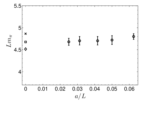
Figure 1: Scaling plot for the pseudoscalar mass $m_{\pi}$.

The results for $Lm_{\pi}$ are plotted in figure 1 against $a/L$. It is clear from the plot that within the 2% errors we do not see any cutoff effect. The symbols at $a/L=0$ correspond to the predictions obtained for our value of the fermion mass from different approximate analytical solutions valid in the limit of small mass and large coupling $g$ [?]. We regard the observed consistency as a check of our setup. In addition, for the same quantity and for a similar choice of parameters, results consistent with lattice artifacts linear in $a^{2}$ have been recently reported also in ref. [?].

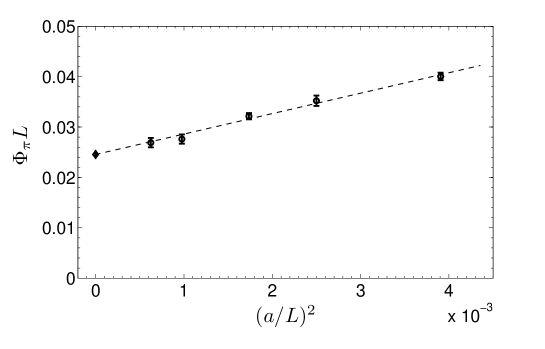
Figure 2: Scaling plot for the matrix element $\Phi_{\pi}$.

The discussion of $L\Phi_{\pi}$ is a bit more delicate since we see cutoff effects in this quantity. As it is shown in figure 2, those are clearly consistent with being linear in $a^{2}$ only. Nevertheless, in order to estimate the size of the O$(am_{\rm q})$ effects, we tried to fit the data also to a polynomial with terms linear and quadratic in $a$. The fit is acceptable in terms of $\chi^{2}$ and the continuum limit we obtain is in agreement with the one in figure 2, but it has a five times larger error. The coefficients of the linear and quadratic terms have large errors as well. They are both consistent with zero but strongly anticorrelated. We conclude that the sensitivity of our data to the O($am_{\rm q}$) effects is very small. Adding a smaller lattice resolution would probably help to disentangle them from the O($a^{2}$).

4. The numerical study presented here confirms the expectation that in the absence of spontaneous chiral symmetry breaking cutoff effects are of O($a^{2}$) also when Wilson fermions are used (at least if the chiral limit is considered). The situation is very different from QCD in four dimensions (and large volume), where for Wilson fermions the O($a$) effects are rather large [?] and have to be removed by following the Symanzik improvement programme [?].

As a consequence, testing fermionic actions by scaling studies in the Schwinger model provides, in our opinion, very little information about the cutoff effects for the same regularizations in the phenomenologically more relevant case of QCD.

On the other hand, to improve our confidence in the argument presented here, it would be interesting to extend the study by considering different values of the fermion mass in order to assess more precisely the size of the residual O($am_{\rm q}$) effects. As far as we can tell now, those appear to be fairly small. In addition, the mass of the scalar particle $\eta$ could be included among the observables. Contrary to the quantities discussed here, this mass does not vanish in the chiral limit [?]. To this end, the numerical techniques introduced in ref. [?] could provide an efficient way to evaluate the contributions coming from disconnected quark diagrams.

Acknowledgments. We thank Francesco Knechtli, Tomasz Korzec, Rainer Sommer and Ulli Wolff for useful discussions. We thank Ulli Wolff for a critical reading of the manuscript. The simulations in the present work have been carried out using the PC cluster at the Humboldt University in Berlin, we thank the staff at the computer center for the assistance. M.D.M. gratefully acknowledges the SFB Transregio 9 for financial support.

References

- [1] K. Symanzik, Some topics in quantum field theory, in: Mathematical problems in theoretical physics, eds. R. Schrader et al., Lecture Notes in Physics, Vol. 153, (Springer, New York, 1982).
- [2] K. Symanzik, Nucl. Phys. B 226 (1983) 187 and 205.
- [3] K. G. Wilson, Phys. Rev. D 10 (1974) 2445.
- [4] M. Lüscher, S. Sint, R. Sommer and P. Weisz, Nucl. Phys. B 478 (1996) 365
- [5] R. Frezzotti and G. C. Rossi, JHEP 0408 (2004) 007.
- [6] S. Aoki and O. Bär, Phys. Rev. D 70 (2004) 116011.
- [7] R. Frezzotti, G. Martinelli, M. Papinutto and G. C. Rossi, hep-lat/0503034.
- [8] J. Schwinger, Phys. Rev 128 (1962) 2425.
- [9] N. D. Mermin and H. Wagner, Phys. Rev. Lett. 17 (1966) 1133.
- [10] F. Knechtli and U. Wolff [Alpha Collaboration], Nucl. Phys. B 663 (2003) 3.
- [11] I. Hip, C. B. Lang and R. Teppner, Nucl. Phys. Proc. Suppl. 63 (1998) 682.
- [12] C. Gattringer, I. Hip and C. B. Lang, Phys. Lett. B 466 (1999) 287.
- [13] B. Sheikholeslami and R. Wohlert, Nucl. Phys. B 259 (1985) 572.
- [14] S. Duane, A. D. Kennedy, B. J. Pendleton and D. Roweth, Phys. Lett. B 195 (1987) 216.
- [15] A. V. Smilga Phys. Rev. D 55 (1997) 443.
- [16] N. Christian, K. Jansen, K. Nagai and B. Pollakowski, hep-lat/0510047.
- [17] M. Lüscher, Advanced Lattice QCD, in: Probing the standard model of particle interactions (Les Houches 1997), eds. R. Gupta et al. (Elsevier, Amsterdam, 1999).
- [18] J. Foley et al., hep-lat/0505023.