DESY 05-210 Edinburgh 2005/17 Second moment of the pion’s distribution amplitude

Abstract

We present preliminary results from the QCDSF/UKQCD collaborations for the second moment of the pion’s distribution amplitude with two flavours of dynamical fermions. We use nonperturbatively determined renormalisation coefficients to convert our results to the $\overline{\rm MS}$ scheme at 5 GeV². Employing a linear chiral extrapolation from our large pion masses $>$ 550 MeV, we find $\langle\xi^{2}\rangle=0.281(28)$, leading to a value of $a_{2}=0.236(82)$ for the second Gegenbauer moment.

1 INTRODUCTION

The distribution amplitude of the pion, $\phi_{\pi}(x,\mu^{2})$, contains information on how the pion’s longitudinal momentum is divided between its quark and anti-quark constituents when probed in diffractive dijet production at E-791 [1] and exclusive pion photoproduction at CLEO [2].

The pion’s distribution amplitude is defined on the light cone as

$$\langle 0|\bar{d}(0)\gamma_{\mu}\gamma_{5}u(z)|\pi^{+}(p)\rangle=$$ (1)

$$\qquad if_{\pi}p_{\mu}\int^{1}_{0}dx\ e^{-ixp\cdot z}\phi_{\pi}(x,\mu)\ ,$$

where $z^{2}=0$ is a vector along the light cone, $x$ is the fraction of the pion’s longitudinal momentum, $p$, carried by the quark ($\bar{x}=1-x$ for the anti-quark), $f_{\pi}$ is the pion decay constant, and $\mu$ is the factorisation scale. On a Euclidean lattice, we are not able to compute matrix elements of bilocal operators such as $\bar{d}(0)\gamma_{\mu}\gamma_{5}u(z)$ in Eq. (1), instead we make use of the light-cone operator product expansion which allows one to calculate Mellin moments of Eq. (1) via the computation of matrix elements of local operators. The $n^{th}$ moment of the pion’s distribution amplitude is defined as

$$\langle\xi^{n}\rangle\equiv\int\ {\rm d}\xi\,\xi^{n}\,\phi(\xi,Q^{2})\ ,$$ (2)

where $\xi\equiv x-\bar{x}=2x-1$, and can be extracted from the matrix elements of twist-2 operators

$$\langle 0|{\cal O}_{\{\mu_{0}\ldots\mu_{n}\}}(0)|\pi(p)\rangle=f_{\pi}p_{\mu_{0}}\ldots p_{\mu_{n}}\langle\xi^{n}\rangle+\cdots\ ,$$ (3)

where

$${\cal O}_{\mu_{0}\ldots\mu_{n}}(0)=(-i)^{n}\overline{\psi}\gamma_{\mu_{0}}\gamma_{5}\stackrel{{\scriptstyle\leftrightarrow}}{{D}}_{\mu_{1}}\ldots\stackrel{{\scriptstyle\leftrightarrow}}{{D}}_{\mu_{n}}\psi\ ,$$ (4)

$\stackrel{{\scriptstyle\leftrightarrow}}{{D}}=\stackrel{{\scriptstyle\rightarrow}}{{D}}-\stackrel{{\scriptstyle\leftarrow}}{{D}}$ and $\{\cdots\}$ denotes symmetrisation of indices and subtraction of traces. We implement the standard normalisation by setting $\langle\xi^{0}\rangle=1$. Due to G-parity the first moment, $\langle\xi^{1}\rangle$, vanishes for the pion, hence the first nontrivial moment that we are able to calculate is $\langle\xi^{2}\rangle$.

Although the first lattice calculations of $\langle\xi^{2}\rangle$ appeared almost 20 years ago [3], there has been surprisingly little activity in this area in recent times [4, 5, 6] to complement other theoretical investigations, e.g. [7, 8, 9, 10, 11, 12, 13, 14, 15, 16, 17, 18]. The current state-of-the-art lattice calculation comes from Del Debbio et al. [6] who performed a simulation in quenched QCD and renormalised their results perturbatively to the $\overline{\rm MS}$ scheme at $\mu=2.67$ GeV, $\langle\xi^{2}\rangle^{\overline{\rm MS}}(\mu=2.67\,{\rm GeV})=0.280(49)^{+0.030}_{-0.013}\ .$

In these proceedings we present preliminary results from the QCDSF/UKQCD collaborations for $\langle\xi^{2}\rangle^{\overline{\rm MS}}$ in two flavour lattice QCD. These results complement our preliminary results on the pion form factor [19].

2 OPERATORS

The $H(4)$ representation on the lattice leads us to consider two operators which we call ${\cal O}^{a}$ and ${\cal O}^{b}$ [20], e.g.

$$\vec{p} = (p,p,0):$$ (5)

$${\cal O}^{a}_{412} ={\cal O}_{\{412\}}\,,$$

$$\vec{p} = (p,0,0):$$ (6)

$${\cal O}^{b}_{411} =\left({\cal O}_{\{411\}}-\frac{{\cal O}_{\{422\}}+{\cal O}_{\{433\}}}{2}\right)\,,$$

where $p=2\pi/L_{s}$ and $L_{s}$ is the spatial extent of our lattice. From Eq. (3), we see that ${\cal O}^{a}$ requires two spatial components of momentum, while ${\cal O}^{b}$ needs only one. Consideration of this fact alone would lead one to choose ${\cal O}^{b}$, since units of momenta in different directions on the lattice lead to a poorer signal. However, lattice operators with two or more covariant derivatives can mix with operators of the same or lower dimension. For forward matrix elements, ${\cal O}^{b}$ suffers from such mixings while ${\cal O}^{a}$ does not. For matrix elements involving a momentum transfer between the two states, i.e. nonforward matrix elements, both operators ${\cal O}^{a}$ and ${\cal O}^{b}$ can mix with operators involving external ordinary derivatives, i.e. operators of the form $\partial_{\mu}\partial_{\nu}\cdots(\bar{\psi}\cdots\psi)$. For example, ${\cal O}^{a}_{412}$ in Eq. (5) can mix with the following operator [20]

$${\cal O}_{\{412\}}^{a,\,\partial\partial}=-\frac{1}{4}\partial_{\{4}\partial_{1}\left(\bar{\psi}\gamma_{2\}}\gamma_{5}\psi\right)\ .$$ (7)

The situation for ${\cal O}^{b}$ is a lot worse as it can potentially mix with up to seven different operators [20]. Hence a complete calculation of $\langle\xi^{2}\rangle$ would require knowledge of the mixing coefficients and renormalisation constants for all of these mixing operators. It now becomes obvious that ${\cal O}^{a}$ offers the best possibility to extract a value of $\langle\xi^{2}\rangle$ from a lattice simulation.

Although the mixing coefficient for ${\cal O}^{a,\,\partial\partial}$ is not yet known, we expect that it is small and hence we anticipate that the contribution to $\langle\xi^{2}\rangle$ from ${\cal O}^{a,\,\partial\partial}$ will be small. Hence, for the rest of the work presented here, we will consider only the contribution from ${\cal O}^{a}$. In a forthcoming publication, we will attempt to address all mixing issues associated with both operators ${\cal O}^{a}$ and ${\cal O}^{b}$.

$\beta$	$\kappa_{\rm sea}$	Volume	$a$ (fm)	$m_{\pi}$ (GeV)
5.20	0.13420	$16^{3}\times 32$	0.1226	0.9407(19)
5.20	0.13500	$16^{3}\times 32$	0.1052	0.7780(24)
5.20	0.13550	$16^{3}\times 32$	0.0992	0.5782(30)
5.25	0.13460	$16^{3}\times 32$	0.1056	0.9217(20)
5.25	0.13520	$16^{3}\times 32$	0.0973	0.7746(25)
5.25	0.13575	$24^{3}\times 48$	0.0904	0.5552(14)
5.29	0.13400	$16^{3}\times 32$	0.1039	1.0952(18)
5.29	0.13500	$16^{3}\times 32$	0.0957	0.8674(17)
5.29	0.13550	$24^{3}\times 48$	0.0898	0.7180(13)
5.29	0.13590	$24^{3}\times 48$	0.0856	0.5513(20)
5.40	0.13500	$24^{3}\times 48$	0.0821	0.9692(14)
5.40	0.13560	$24^{3}\times 48$	0.0784	0.7826(17)
5.40	0.13610	$24^{3}\times 48$	0.0745	0.5856(22)

Table 1: Lattice parameters: Gauge coupling $\beta$, sea quark hopping parameter $\kappa_{\rm sea}$, lattice volume, lattice spacing and pion mass.

3 LATTICE TECHNIQUES

We simulate with $N_{f}=2$ dynamical configurations generated with Wilson glue and nonperturbatively ${\cal O}(a)$ improved Wilson fermions. For four different values $\beta=5.20$, $5.25$, $5.29$, $5.40$ and up to four different kappa values per beta we have generated ${\cal O}(2000-8000)$ trajectories. Lattice spacings and spatial volumes vary between 0.075-0.123 fm and (1.5-2.2 fm)³ respectively. A summary of the parameter space spanned by our dynamical configurations can be found in Table 1. We set the scale via the force parameter, with $r_{0}=0.5$ fm.

Correlation functions are calculated on configurations taken at a distance of 10 trajectories using 4 different locations of the fermion source. We use binning to obtain an effective distance of 20 trajectories. The size of the bins has little effect on the error, which indicates residual auto-correlations are small.

We calculate the average of matrix elements computed with three choices of pion momenta $\vec{p}_{0}=(p,p,0)$, $\vec{p}_{1}=(p,0,p)$, $\vec{p}_{2}=(0,p,p)$, with the indices of the operators (Eq. (5)) chosen accordingly.

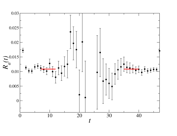
Figure 1: Ratio defined in Eq. (9), using ${\cal O}^{a}$ from Eq. (5), on a $24^{3}\times 48$ lattice with $\beta=5.40$ and $\kappa_{\rm sea}=0.13560$.

We define a pion two-point correlation function as

$$C^{\cal O}(t,\vec{p})=\sum_{\vec{x}}e^{i\vec{p}\cdot\vec{x}}\left\langle{\cal O}(\vec{x},t)J(\vec{0},0)^{\dagger}\right\rangle\ ,$$ (8)

$$\rightarrow \frac{Z}{2E}\langle 0|{\cal O}(0)|\pi(p)\rangle e^{-Et},\ \ t\gg 0\,,$$

where $Z=\langle\pi(p)|J(0)^{\dagger}|0\rangle$ and we use $J(x)\equiv\pi(x)=\overline{\psi}(x)\gamma_{5}\psi(x)$ as the interpolating operator for the pion. The matrix elements in Eq. (3) are then extracted from the following ratios of two-point functions,

$$R^{a} = \frac{C^{{\cal O}^{a}_{4ij}}(t)}{C^{{\cal O}_{4}}(t)}=p_{i}p_{j}\ \langle\xi^{2}\rangle^{a}\ ,$$ (9)

$$R^{b} = \frac{C^{{\cal O}^{b}_{4ii}}(t)}{C^{{\cal O}_{4}}(t)}=p_{i}^{2}\ \langle\xi^{2}\rangle^{b}\ ,$$ (10)

where $i$ and $j$ are spatial indices, and ${\cal O}_{4}$ is the operator given in Eq. (4) with no derivatives and $\mu_{0}=4$.

Figure 1 shows a typical example of the ratio in Eq. (9) where we clearly observe two plateaus for $t<L_{T}/2$ and $t>L_{T}/2$, where $L_{T}$ is the time extent of the lattice. After extracting $R^{a}$ from the plateaus, we use Eq. (9) to extract $\langle\xi^{2}\rangle$.

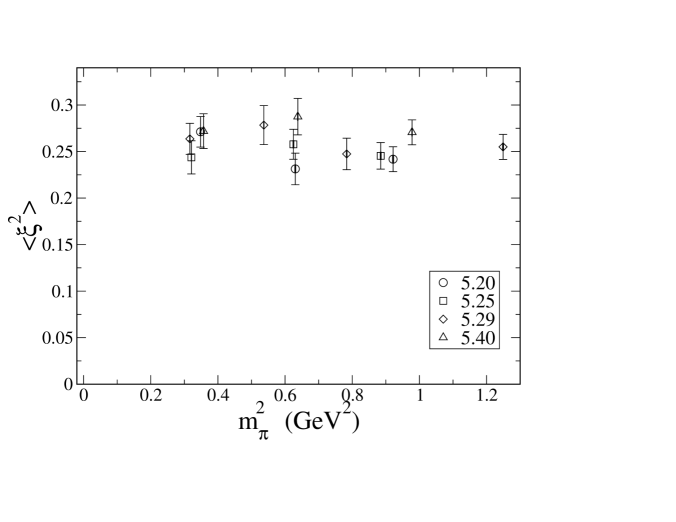
Figure 2: $\langle\xi^{2}\rangle$ as a function of $m_{\pi}^{2}$ for ${\cal O}^{a}$ from Eq. (5).

In general, bare lattice operators must be renormalised in some scheme, ${\cal S}$, and at a scale, $M$,

$${\cal O}^{\cal S}(M)=Z^{\cal S}_{\cal O}(M){\cal O}_{\rm bare}\ ,$$ (11)

so in order to calculate a renormalised value for $\langle\xi^{2}\rangle$, we must consider

$$\langle\xi^{2}\rangle^{\cal S}(M)=\frac{Z^{\cal S}_{\cal O}(M)}{Z_{{\cal O}_{4}}}\langle\xi^{2}\rangle_{\rm bare}\ .$$ (12)

We choose to renormalise to the $\overline{\rm MS}$ scheme at a scale of $\mu^{2}=5\,{\rm GeV}^{2}$. Further details of our renormalisation techniques can be found in [21] and a forthcoming publication.

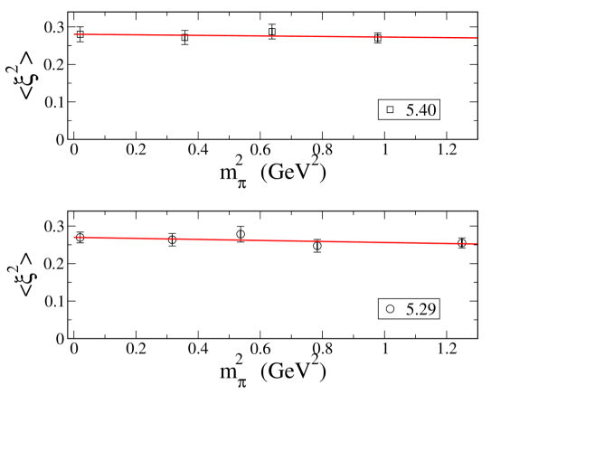
Figure 3: Chiral extrapolation at constant $\beta$ for $\beta=5.40$ (top) and $\beta=5.29$ (bottom) for ${\cal O}^{a}$ from Eq. (5).

4 RESULTS FOR $\langle\xi^{2}\rangle$

For each of our datasets, we extract a value for $\langle\xi^{2}\rangle_{\rm bare}$ from Eq. (9) and renormalise using Eq. (12). Figure 2 shows these results plotted as a function of $m_{\pi}^{2}$. Here we observe that the results are approximately constant as we vary the pion mass.

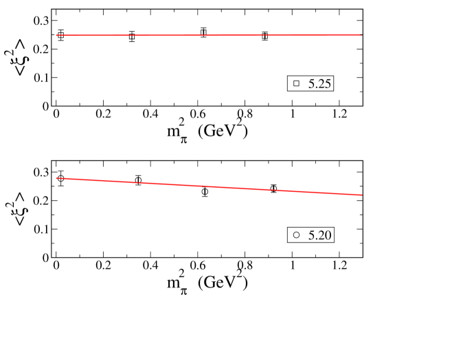
Figure 4: Chiral extrapolation at constant $\beta$ for $\beta=5.25$ (top) and $\beta=5.20$ (bottom) for ${\cal O}^{a}$ from Eq. (5).

In order to obtain a result in the continuum and chiral limits, we first extrapolate our results at constant $\beta$ to the chiral limit. In Fig. 3 we display the chiral extrapolations for $\beta=5.40$ (top) and 5.29 (bottom), while Fig. 4 contains the corresponding extrapolations for $\beta=5.25$ (top) and 5.20 (bottom). These results exhibit only a mild dependence on the quark mass and their values in the chiral limit agree within errors.

Now that we have calculated results in the chiral limit for each choice of $\beta$, we are in a position to examine the behaviour of our results as a function of the lattice spacing. In Fig. 5 we use the values of $r_{0}$ calculated in the chiral limit for each $\beta$ (see Table 3 of Ref. [22]) to study the dependence of our results on the lattice spacing. Here we observe that even though our operators are not ${\cal O}(a)$-improved, we find a negligible dependence on the lattice spacing, at least when compared to the statistical errors. Hence we take the result at our smallest lattice spacing (largest $\beta$) as our result in the continuum limit.

We find in the continuum limit at the physical pion mass, the second moment of the pion’s distribution amplitude to be

$$\langle\xi^{2}\rangle^{\overline{\rm MS}}(\mu^{2}=5\,{\rm GeV}^{2})=0.281(28)\ ,$$ (13)

which is very close to the value $\langle\xi^{2}\rangle^{\overline{\rm MS}}(\mu=2.67\,{\rm GeV})=0.280(49)^{+0.030}_{-0.013}$ found in Ref. [6], and larger than the asymptotic value, $\mu^{2}\rightarrow\infty$

$$\phi_{\rm as}(\xi)=\frac{3}{2}(1-\xi^{2})\ \Rightarrow\ \langle\xi^{2}\rangle=0.2\ .$$ (14)

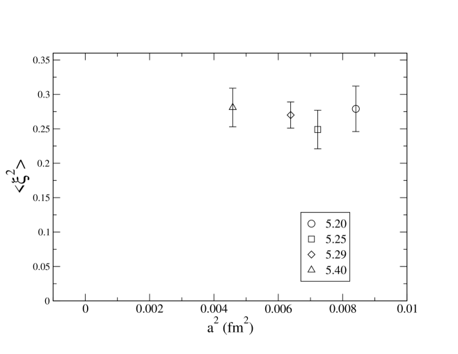
Figure 5: Results for each value of $\beta$ in the chiral limit as a function of $a^{2}$ for ${\cal O}^{a}$ from Eq. (5).

5 GEGENBAUER MOMENT $a_{2}$

The distribution amplitude, $\phi(x,\mu^{2})$, can be expanded in a series of even Gegenbauer polynomials, $C_{2n}^{\frac{3}{2}}(2x-1)$ [8, 9],

$$\phi(x,\mu^{2})=6x(1-x)\sum_{n=0}^{\infty}a_{2n}(\mu^{2})C_{2n}^{\frac{3}{2}}(2x-1),$$ (15)

where $a_{2n}(\mu^{2})$ are the multiplicatively renormalisable Gegenbauer moments. Since the higher moments, $n>4$, are expected to be small, it is common to truncate Eq. (15)

$$\phi(x,\mu^{2}) = 6x(1-x)\left\{1+a_{2}(\mu^{2})C_{2}^{\frac{3}{2}}(2x-1)\right.$$ (16)

$$+ \left.a_{4}(\mu^{2})C_{4}^{\frac{3}{2}}(2x-1)\right\}\,.$$

In the asymptotic limit, $\mu^{2}\rightarrow\infty$, all $a_{2n}(\mu^{2})=0$, for $n>0$.

Analyses of CLEO data for $F_{\pi\gamma\gamma^{*}}$ constrain the pion distribution amplitude by calculating a relationship between the first two Gegenbauer moments (see eg., [15, 16]), together with upper and lower bounds on their respective values.

Taking the second $\xi=2x-1$ moment of the r.h.s. of Eq. (16) gives

$$\langle\xi^{2}\rangle=\int^{1}_{0}d\xi\ \xi^{2}\phi(\xi,\,\mu^{2})=\frac{1}{35}\left(7+12a_{2}(\mu^{2})\right)\,,$$ (17)

which allows us to extract $a_{2}$, but not $a_{4}$. In order to place a constraint on $a_{4}$, we would need to calculate the fourth moment of the pion’s distribution amplitude which requires using an operator involving four covariant derivatives.

Using our result in Eq. (13) we calculate

$$a_{2}(\mu^{2}=5\,{\rm GeV}^{2})=0.236(82)\ ,$$ (18)

which is larger than the values $a_{2}(1\,{\rm GeV})=0.07(1)$ [17] and $a_{2}(1\,{\rm GeV})=0.19(19)$ [18], but within the usual constraints $0\leq a_{2}(1\,{\rm GeV})\leq 0.3$ commonly quoted in the literature, even when we consider that our value will increase slightly when we run our result to a smaller scale of $\mu=1$ GeV.

6 CONCLUSIONS

We have presented a preliminary result for the second moment of the pion’s distribution amplitude calculated on lattices generated by the QCDSF/UKQCD collaboration with two flavours of dynamical fermions. We use nonperturbatively determined renormalisation coefficients to convert our result to the $\overline{\rm MS}$ scheme at 5 GeV². We find $\langle\xi^{2}\rangle=0.281(28)$, which is very close to an earlier lattice result and larger than the asymptotic value.

Using a fourth order Gegenbauer polynomial expansion, we calculate a value for the second Gegenbauer moment, $a_{2}(\mu^{2}=5\,{\rm GeV}^{2})=0.236(82)$.

Although we have only employed a linear chiral extrapolation and our operators are not ${\cal O}(a)$-improved, the chiral and continuum extrapolations do not seem to be a major source of systematic error when compared to the statistical errors. These issues will be addressed in more detail in a forthcoming coming publication, where we also intend to investigate finite size and (partially) quenching effects as well as renormalisation group running of the relevant matrix elements.

References

- [1] E. M. Aitala et al. [E791 Collaboration], Phys. Rev. Lett. 86, 4768 (2001) [arXiv:hep-ex/0010043].
- [2] J. Gronberg et al. [CLEO Collaboration], Phys. Rev. D 57, 33 (1998) [arXiv:hep-ex/9707031].
- [3] A. S. Kronfeld and D. M. Photiadis, Phys. Rev. D 31, 2939 (1985); G. Martinelli and C. T. Sachrajda, Phys. Lett. B 190, 151 (1987).
- [4] D. Daniel, R. Gupta and D. G. Richards, Phys. Rev. D 43, 3715 (1991).
- [5] L. Del Debbio, M. Di Pierro, A. Dougall and C. T. Sachrajda [UKQCD collaboration], Nucl. Phys. Proc. Suppl. 83, 235 (2000) [arXiv:hep-lat/9909147].
- [6] L. Del Debbio, M. Di Pierro and A. Dougall [UKQCD collaboration], Nucl. Phys. Proc. Suppl. 119, 416 (2003) [arXiv:hep-lat/0211037].
- [7] V. L. Chernyak and A. R. Zhitnitsky, Phys. Rept. 112, 173 (1984).
- [8] V. M. Braun and I. E. Filyanov, Z. Phys. C 48, 239 (1990) [Sov. J. Nucl. Phys. 52, 126 (1990)].
- [9] V. M. Braun, G. P. Korchemsky and D. Müller, Prog. Part. Nucl. Phys. 51, 311 (2003) [arXiv:hep-ph/0306057].
- [10] P. Ball, JHEP 9901, 010 (1999) [arXiv:hep-ph/9812375].
- [11] P. Ball and M. Boglione, Phys. Rev. D 68, 094006 (2003) [arXiv:hep-ph/0307337].
- [12] A. P. Bakulev, S. V. Mikhailov and N. G. Stefanis, Phys. Lett. B 508, 279 (2001) [Erratum-ibid. B 590, 309 (2004)] [arXiv:hep-ph/0103119].
- [13] A. Schmedding and O. I. Yakovlev, Phys. Rev. D 62, 116002 (2000) [arXiv:hep-ph/9905392].
- [14] A. P. Bakulev, K. Passek-Kumericki, W. Schroers and N. G. Stefanis, Phys. Rev. D 70, 033014 (2004) [Erratum-ibid. D 70, 079906 (2004)] [arXiv:hep-ph/0405062].
- [15] M. Diehl, P. Kroll and C. Vogt, Eur. Phys. J. C 22, 439 (2001) [arXiv:hep-ph/0108220].
- [16] A. P. Bakulev, S. V. Mikhailov and N. G. Stefanis, Phys. Rev. D 67, 074012 (2003) [arXiv:hep-ph/0212250].
- [17] S. Dalley and B. van de Sande, Phys. Rev. D 67, 114507 (2003) [arXiv:hep-ph/0212086].
- [18] P. Ball and R. Zwicky, Phys. Lett. B 625, 225 (2005) [arXiv:hep-ph/0507076].
- [19] D. Brömmel, M. Diehl, M. Göckeler, Ph. Hägler, R. Horsley, D. Pleiter, P. E. L. Rakow, A. Schäfer, G. Schierholz and J. M. Zanotti [QCDSF Collaboration], arXiv:hep-lat/0509133.
- [20] M. Göckeler, R. Horsley, H. Perlt, P. E. L. Rakow, A. Schäfer, G. Schierholz and A. Schiller [QCDSF Collaboration], Nucl. Phys. B 717, 304 (2005) [arXiv:hep-lat/0410009].
- [21] M. Göckeler, R. Horsley, D. Pleiter, P. E. L. Rakow and G. Schierholz [QCDSF Collaboration], Phys. Rev. D 71, 114511 (2005) [arXiv:hep-ph/0410187].
- [22] M. Göckeler, R. Horsley, A. C. Irving, D. Pleiter, P. E. L. Rakow, G. Schierholz and H. Stüben [QCDSF Collaboration], arXiv:hep-ph/0502212.
- [23] C. R. Allton et al. [UKQCD Collaboration], Phys. Rev. D 65, 054502 (2002) [arXiv:hep-lat/0107021].