The QCD phase diagram at finite density
                                                                                                 BNL-NT-05/38
                                                                                                 WUB-05-12
                                                                                                 ITP-Budapest 623

Abstract:

We study the density of states method to explore the phase diagram of the chiral transition on the tempeature and quark chemical potential plane. Four quark flavours are used in the analysis. Though the method is quite expensive small lattices show an indication for a triple-point connecting three different phases on the phase diagram.

PoS(LAT2005)163

1 Introduction

To clarify the phase diagram of QCD and thus the nature of matter under extreme conditions is one of the most interesting and fundamental tasks of high energy physics. Lattice QCD has been shown to provide important and reliable information from first principals on QCD at zero density. However, Lattice QCD at finite densities has been harmed by the complex action problem ever since its inception. For $\mu>0$ the determinant of the fermion matrix ($\rm{det}M$) becomes complex. Standard Monte Carlo techniques using importance sampling are thus no longer applicable when calculating observables in the grand canonical ensemble according to the partition function

$$Z_{GC}(\mu)=\int\mathcal{D}U\;\rm{det}M[U](\mu)\exp\{-S_{G}[U]\}.$$ (1)

Recently many different methods have been developed to cirumvent the complex action problem for small $\mu/T$ [1, 2]. For a recent overview see also [3].

2 Formulation of the method

A very general formulation of the DOS method is the following: One exposed parameter ($\phi$) is fixed. The expectation value of a thermodynamic observable ($O$), according to the usual grand canonical partition function (1), can be recovered by the integral

$$<O>=\int d\phi\,\left<Of(U)\right>_{\phi}\rho(\phi)\left/\int d\phi\,\left<f(U)\right>_{\phi}\rho(\phi)\right.$$ (2)

where the density of states ($\rho$) is given by the constrained partition function:

$$\rho(x)\equiv Z_{\phi}(x)=\int\mathcal{D}U\,g(U)\,\delta(\phi-x).$$ (3)

With $\left<~{}\right>_{\phi}$ we denote the expectation value with respect to the constrained partition function. In addition, the product of the weight functions $f,g$ has to give the correct measure of $Z_{GC}$: $fg=\rm{det}M\exp\{-S_{G}\}$. This idea of reordering the partition functions is rather old and was used in many different cases [4, 5, 6] The advantages of this additional integration becomes clear, when choosing $\phi=P$ and $g(U)=1$. In this case $\rho(\phi)$ is independent of all simulation parameters. The observable can be calculated as a function of all values of the lattice coupling $\beta$. If one has stored all eigenvalues of the fermion matrix for all configurations, the observable can also be calculated as a function of quark mass ($m$) and number of flavors[5] ($N_{f}$). In this work we chose

$$\phi=P\qquad\mbox{and}\qquad g=\left|{\rm det}M\right|\exp\{-S_{G}\},\qquad f=\exp\{i\theta\}.$$ (4)

In other words we constrain the plaquette and perform simulations with measure $g$. In practice, we replace the delta function in Equation (3) by a sharply peaked potential [6]. The constrained partition function for fixed values of the plaquette expectation value can then be written as

$$\rho(x)\approx\int{\cal D}U\;g(U)\exp\left\{-V(x)\right\},$$ (5)

where $\exp\{-V(x)\}$ is a Gaussian potential with

$$V(x)=\frac{1}{2}\gamma\left(x-P\right)^{2}.$$ (6)

We obtain the density of states ($\rho(x)$) by the fluctuations of the actual plaquette $P$ around the constraint value $x$. The fluctuation dissipation theorem gives

$$\frac{d}{dx}\ln\rho(x)=<x-P>_{x}.$$ (7)

Before performing the integrals in Equation (2) we compute from an ensemble generated at $(\mu_{0},\beta_{0})$:

$$\left<Of(U)\right>_{x}(\mu,\beta) = \left<Of(U)R(\mu,\mu_{0},\beta,\beta_{0})\right>_{x}/\left<R(\mu,\mu_{0},\beta,\beta_{0})\right>_{x},$$ (8)

$$\left<f(U)\right>_{x}(\mu,\beta) = \left<f(U)R(\mu,\mu_{0},\beta,\beta_{0})\right>_{x}/\left<R(\mu,\mu_{0},\beta,\beta_{0})\right>_{x},$$ (9)

$$\frac{d}{dx}\ln\rho(x,\mu,\beta) = \left<(x-P)R(\mu,\mu_{0},\beta,\beta_{0})\right>_{x}.$$ (10)

Here $R$ is given by the quotient of the measure $g$ at the point $(\mu,\beta)$ and at the simulation point $(\mu_{0},\beta_{0})$,

$$R(\mu,\mu_{0},\beta,\beta_{0})=g(\mu,\beta)/g(\mu_{0},\beta_{0})=\frac{|{\rm det}(\mu)|}{|{\rm det}(\mu_{0})|}\exp\{S_{G}(\beta)-S_{G}(\beta_{0})\}.$$ (11)

Heaving calculated the expressions (8)-(10), we are able to extrapolate the expectation value of the observable (2) to any point $(\mu,\beta)$ in a small region around the simulation point $(\mu_{0},\beta_{0})$. For any evaluation of $\left<O\right>(\mu,\beta)$, we numerically perform the integrals in Equation (2). We also combine the data from several simulation points to interpolate between them.

3 Simulations with constrained plaquette

The value we want to constrain is the expectation value of the global plaquette, which is given on every gauge configuration by the sum over all lattice points ($y$) and directions ($\mu\nu$) of the local plaquette $P_{\mu\nu}(y)$ and its adjoint $P^{\dagger}_{\mu\nu}(y)$,

$$P=\sum_{y}\sum_{1\leq\mu<\nu\leq 4}\frac{1}{6}\left[{\rm Tr}P_{\mu\nu}(y)+{\rm Tr}P^{\dagger}_{\mu\nu}(y)\right].$$ (12)

Since the plaquette is also the main part of the gauge action,

$$S_{G}=-\beta\sum_{x}\sum_{1\leq\mu<\nu\leq 4}\left\{\frac{1}{6}\left[{\rm Tr}P_{\mu\nu}(x)+{\rm Tr}P^{\dagger}_{\mu\nu}(x)\right]-1\right\},$$ (13)

the additional potential $V$ can be easily introduced in the hybrid Monte Carlo update procedure of the hybrid-R algorithm [7]. After calculating the equation of motion for the link variables $U_{\mu}(y)$, we find for the gauge part of the force

$$i\dot{H}_{\mu}(y)=\left[\frac{\beta}{3}U_{\mu}(y)T_{\mu}(y)\left(1+\frac{\gamma(x-P)}{\beta}\right)\right]_{\rm TA}.$$ (14)

Here the subscript ${\rm TA}$ indicates the traceless anti-Hermitian part of the matrix. We see that in each molecular dynamical step the measurement of the plaquette is required. However, the only modification in the gauge force is the factor in round brackets.

4 The critical line and the determination of a triple-point

Simulations have been performed with staggered fermions and $N_{f}=4$. We chose 9 differed points in the $(\beta,\mu)$-plane for the $4^{4}$ lattice and 8 points for the $6^{4}$ lattice. On each of these points we did simulations with 20-40 constrained plaquette values, all with quark mass $am=0.05$. Further simulations has been done with $(\beta,\mu)=(5.1,0.3)$ on the $6^{3}\times 8$ lattice for $am=0.05$ and $am=0.03$.

Fist of all we check, whether we can reproduce old results with our new method. We show in Figure 1(a) results from a Simulation at $\mu=0.3$, $\beta=4.98$ and $\lambda=0.02$.

(a)

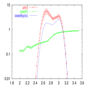
(b)

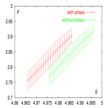
(c)

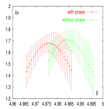
(d)

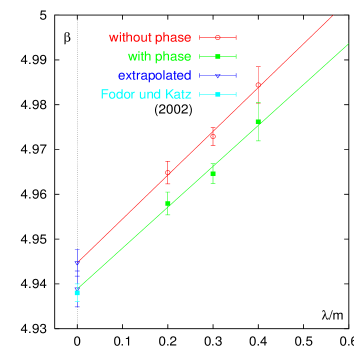
Figure 1: Results for Simulations at $\beta=4.98$, $\mu=0.3$, $\lambda=0.02$, $n_{f}=4$, $am=0.05$, and number of lattice points: $4^{4}$. Shown are: (a) the density of states $\rho(x)$, the phase factor $\left<\cos(\theta)\right>$, and their product, (b) the Plaquette as a function of the coupling $\beta$, with and without the phase factor, (c) the Susceptibility of the Plaquette as a function of the coupling $\beta$, with and without the phase factor, and (d) the extrapolation $\beta_{c}(\lambda)$ to $\lambda=0$, with and without the phase factor.

Here we plot the density of states ($\rho$) and the real part of the phase factor $\left<cos(\theta)\right>$ as a function of the constrained plaquette value. The results have been interpolated in $P$, in order to obtain a better result for the necessary integration over $P$. The distribution $\rho$ shows a clear double peak structure, which signals the transition. The phase factor is smaller in the low temperature phase ($P\raise 1.29167pt\hbox{$<$\kern-7.5pt\raise-4.73611pt\hbox{$\sim$}}2.8$). Hence in the product $\rho\left<cos(\theta)\right>$ the low temperature peak is suppressed. Now we perform the integrals

$$\left<P\right>=\int dx\;x\rho(x)\left<cos(\theta)\right>_{x},\qquad\left<P^{2}\right>=\int dx\;x^{2}\rho(x)\left<cos(\theta)\right>_{x}.$$ (15)

In Figure 1(b) we plot the plaquette expectation value $\left<P\right>$ as a function of the coupling $\beta$. The $\beta$-dependence is given by Equations (8)-(10). We indeed find that including the phase factor does shift the transition to lower values of the coupling, which also means to lower temperatures. This can also be seen in a shift of the peak of the susceptibility of the plaquette $\chi_{P}\equiv\left<P^{2}\right>-\left<P\right>^{2}$, which we plot in Figure 1(c). Since the $\lambda$ parameter introduces a systematic error, which can be seen by the relative large critical coupling of $\beta_{c}=4.976(4)$ in comparison to the result form multi-parameter reweighting $\beta_{c}=4.938(2)$ [1], we perform the a linear extrapolation of $\lambda\to 0$, from $\lambda=0.02$, $\lambda=0.015$ and $\lambda=0.01$. We show the extrapolation in Figure 1(d). The extrapolated result $\beta=4.938(4)$ (including the phase factor) and the result from multi-parameter reweighting are in very good agreement. From now on we only give results for $\lambda/m=0.2$, the $\lambda$ dependence is however expected to be smaller for larger $\mu$.

In the range of $0.4\raise 1.29167pt\hbox{$<$\kern-7.5pt\raise-4.73611pt\hbox{$\sim$}}a\mu\raise 1.29167pt\hbox{$<$\kern-7.5pt\raise-4.73611pt\hbox{$\sim$}}0.5$ for the $4^{4}$ lattice, as well as $0.3\raise 1.29167pt\hbox{$<$\kern-7.5pt\raise-4.73611pt\hbox{$\sim$}}a\mu\raise 1.29167pt\hbox{$<$\kern-7.5pt\raise-4.73611pt\hbox{$\sim$}}0.4$ for the $6^{4}$ lattice we found two transitions in the plaquette expectation value $\left<P\right>(\beta)$. The two critical couplings result in two transition lines in the phase diagram. The two transition lines are almost perpendicular in the ($\beta,\mu$)-diagram, and join in a triple-point of the phase diagram. in Figure 2(a) we show the phase diagram in physical units.

(a)

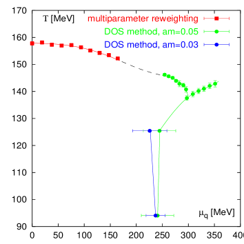
(b)

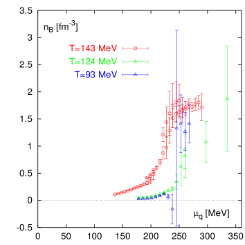
Figure 2: The phase diagram in physical (a), and the quark number density at constant temperature $T=143~{}\mbox{MeV}$ ($4^{4}$ lattice), $T=124~{}\mbox{MeV}$ ($6^{4}$ lattice) and $T=93~{}\mbox{MeV}$ ($6^{3}\times 8$ lattice).

The scale was set by the Sommer radius $r_{0}$, measured on a $10^{3}\times 20$ lattice. In both cases, the triple point is located around $\mu_{q}^{\rm tri}\approx 300~{}\mbox{MeV}$, however its temperature ($T^{\rm tri}$) decreases from $T^{\rm tri}\approx 148\mbox{MeV}$ on the $4^{4}$ lattice to $T^{\rm tri}\approx 137\mbox{MeV}$ on the $6^{4}$ lattice.

Also shown in Figure 2(a) are points from simulations with quark mass $am=0.03$. The phase boundary turned out to be — within our statistical uncertainties — independent of the the mass.

5 The quark number density

To reveal the properties of the new phase located in the lower right corner of the phase diagram, we calculated the quark number density, at constant coupling $\beta$ and at constant temperature respectively. To obtain the density $n_{q}$ we perform the following integration

$$\left<\frac{{\rm d}\ln{\rm det}M}{{\rm d}(a\mu)}\right>=\int dx\;\left<\frac{{\rm d}\ln{\rm det}M}{{\rm d}(a\mu)}cos(\theta)\right>_{x}\rho(x)$$ (16)

The thermodynamic quantity $n_{q}$ are given as usual by

$$n_{q}=\frac{1}{a^{3}N_{s}^{3}N_{t}}\left<\frac{{\rm d}\ln{\rm det}M}{{\rm d}(a\mu)}\right>$$ (17)

In Figure 2(b) we show the baryon number density, which is related to the quark number density by $n_{B}=n_{q}/3$. The results are plotted in physical units and correspond to a constant temperature of $T\approx 143~{}\mbox{MeV}$ ($4^{4}$ lattice), $T\approx 124~{}\mbox{MeV}$ ($6^{4}$ lattice) and $T\approx 93~{}\mbox{MeV}$ ($6^{4}\times 8$ lattice). In order to divide out the leading order cut-off effect, we multiply we have multiplied the data with the factor $c=SB(N_{t})/SB$, which is the Stefan-Boltzmann value of a free lattice gas of quarks at a given value of $N_{t}$, divided by its continuum Stefan-Boltzmann value. At the same value of the chemical potential where we find also a peak in the susceptibility of the plaquette ($\mu_{c})$, we see a sudden rise in the baryon number density. Thus for $\mu>\mu_{c}$ we enter a phase of dense matter. The transition occurs at a density of $(2-3)\times n_{N}$, where $n_{N}$ denotes nuclear matter density. Above the transition, the density reaches values of $(10-20)\times n_{N}$. Quite similar results have been obtained recently by simulations in the canonical ensemble [8].

References

- [1] Z. Fodor and S. D. Katz, Phys. Lett. B534 (2002) 87 [hep-lat/0104001].
- [2] Z. Fodor and S. D. Katz, JHEP 0203 (2002) 014; C. R. Allton et al., Phys. Rev. D66 (2002) 074507; R. V. Gavai and S. Gupta, Phys. Rev. D 68 (2003) 034506; P. R. Crompton, [hep-lat/0301001]; M. D’Elia and M. P. Lombardo, Phys. Rev. D67 (2003) 014505; P. de Forcrand and O. Philipsen, Nucl. Phys. B642 (2002) 290; Nucl. Phys. B673 (2003) 170; V. Azcotiti, et al., [hep-lat/0503010].
- [3] O. Philipsen, these proceedings.
- [4] G. Bhanot, K. Bitar and R. Salvador, Phys. Lett. B187 (1987) 381; Phys. Lett. B188 (1987) 246; M. Karliner, S.R. Sharpe and Y.F. Chang, Nucl. Phys. B302 (1988) 204; V. Azcoiti, G. di Carlo and A. F. Grillo, Phys. Rev. Lett. 65 (1990) 2239; A. Gocksch, Phys. Rev. Lett. 61 (1988) 2054.
- [5] X. Q. Luo, Mod. Phys. Lett. A16 (2001) 1615.
- [6] J. Ambjorn, K. N. Anagnostopoulos, J. Nishimura and J. J. M. Verbaarschot, JHEP 0210 (2002) 062.
- [7] S. Gottlieb, W. Liu, D. Toussaint, R. L. Renken and R. L. Sugar, Phys. Rev. B35 (1987) 2531.
- [8] A. Alexandru, M. Faber, I. Horvath and K. F. Liu, [hep-lat/0410002].