Unified chiral analysis of the vector meson spectrum from lattice QCD

Abstract

The chiral extrapolation of the vector meson mass calculated in partially-quenched lattice simulations is investigated. The leading one-loop corrections to the vector meson mass are derived for partially-quenched QCD. A large sample of lattice results from the CP-PACS Collaboration is analysed, with explicit corrections for finite lattice spacing artifacts. To incorporate the effect of the opening decay channel as the chiral limit is approached, the extrapolation is studied using a necessary phenomenological extension of chiral effective field theory. This chiral analysis also provides a quantitative estimate of the leading finite volume corrections. It is found that the discretisation, finite-volume and partial quenching effects can all be very well described in this framework, producing an extrapolated value of $M_{\rho}$ in excellent agreement with experiment. This procedure is also compared with extrapolations based on polynomial forms, where the results are much less enlightening.

LABEL:FirstPage1 LABEL:LastPage#12

I Introduction

There has been great progress in lattice QCD in recent years, associated both with Moore’s Law and with improved algorithms, which mean that one can work with larger lattice spacings and still approximate the continuum limit well. The CP-PACS group has devoted considerable effort to the study of the masses of the lowest mass baryons and vector mesons. This has led, for example, to a comprehensive set of data for the mass of the $\rho$-meson in partially quenched QCD, with exceptionally small statistical errors cppacs . We shall exploit this data.

The remaining barrier to direct comparison with experimental data is the fact that calculations take much longer as the quark mass approaches the chiral limit. Indeed the time for a given calculation scales somewhere in the range $m_{\pi}^{-7}$ to $m_{\pi}^{-9}$, depending on how hard one works to preserve chiral symmetry. As a result there has been considerable interest in using chiral perturbation theory ($\chi$PT), an effective field theory (EFT) built on the symmetries of QCD, to provide a functional form for hadron properties as a function of quark mass Leinweber:2003dg ; Procura:2003ig . In principle, such a functional form can then be used to extrapolate from the large pion masses where lattice data exists to the physical value. Unfortunately, there is considerable evidence that the convergence of dimensionally regularised $\chi$PT is too slow for this expansion to be reliable at present Leinweber:1999ig ; Bernard:2002yk ; Young:2002ib ; Durr:2002zx ; Beane:2004ks ; Thomas:2004iw ; Leinweber:2005xz .

On the other hand, it can be shown that a reformulation of $\chi$PT using finite-range regularisation (FRR) effectively resums the chiral expansion, leaving a residual series with much better convergence properties Leinweber:2003dg ; Young:2002ib . The FRR expansion is mathematically equivalent to dimensionally regularised $\chi$PT to the finite order one is working Donoghue:1998bs ; Young:2002ib . Systematic errors associated with the functional form of the regulator are at the fraction of a percent level Leinweber:2003dg . A formal description of the formulation of baryon $\chi$PT using a momentum cutoff (or FRR) has recently been considered by Djukanovic et al. Djukanovic:2005jy . The price of such an approach is a residual dependence on the regulator mass, which governs the manner in which the loop integrals vanish as the pion mass grows large. However, if it can be demonstrated that reasonable variation of this mass does not significantly change the extrapolated values of physical properties, one has made progress. This seems to be the case for the nucleon mass Thomas:2004iw and magnetic moments Young:2004tb , for example, where “reasonable variation” is taken to be $\pm$20% around the best fit value of the optimal regulator mass.

In order to test whether the problem is indeed solved in this way one needs a large body of accurate data. This is in fact available for the $\rho$ meson, where CP-PACS has carried out lattice simulations of partially quenched QCD (pQQCD) with a wide range of sea and valence masses. This sector requires a modified effective field theory, namely partially-quenched chiral perturbation theory (PQ$\chi$PT) Golterman:1997st ; Sharpe:2001fh . Formal developments in this field have made significant progress in the study of a range of hadronic observables — see Refs. Chen:2001yi ; Beane:2002vq ; Leinweber:2002qb ; Arndt:2003ww ; Arndt:2004bg ; Bijnens:2004hk ; Detmold:2005pt for example.

In considering the $\rho$ meson, analysis of modern lattice results requires one to extend beyond the low-energy EFT. Near the chiral limit, the $\rho$ decays to two energetic pions, whereas at the quark-masses simulated on the lattice the $\rho$ is stable. The pions contributing to the imaginary part of the $\rho$ mass cannot be considered soft, and therefore cannot be systematically incorporated into a low-energy counting scheme Bijnens:1997ni ; Bruns:2004tj . Because almost all the lattice simulation points in this analysis lie in the region $m_{\pi}>m_{\rho}/2$, it is evident that the extrapolation to the chiral regime will encounter a threshold effect where the decay channel opens. To incorporate this physical threshold, we model the $\rho\to\pi\pi$ self-energy diagram constrained to reproduce the observed width at the physical pion mass. Including this contribution also provides a model of the finite volume corrections arising from the infrared component of the loop integral. In particular, we can also describe the lattice results in the region $m_{\pi}<m_{\rho}/2$, where the decay channel is still energetically forbidden because of momentum discretisation.

This large body of pQQCD simulation data is analysed within a framework which incorporates the leading low-energy behaviour of partially-quenched EFT, together with a model for describing the decay channel of the $\rho$ meson. Finite-range regularisation is implemented to evaluate loop integrals, for reasons discussed above. The aim is to test whether it produces a more satisfactory description of the complete data set than the more commonly used, naive extrapolation formulas. A condensed version of some the work featured here has been reported in Ref. Allton:2005fb .

The next section summarises the finite-range regularised forms for the self-energy of the $\rho$ meson in the case of pQQCD. Section III discusses the data used from the CP-PACS Collaboration cppacs . We then give details of the chiral fits in Sec. IV. Finally, Sec. V reports the experimental determination of the $\rho$ meson mass at the physical point.

II Self-Energies for the Partially Quenched Analysis

Theoretical calculations of dynamical-fermion QCD provide an opportunity to explore the properties of QCD in an expansive manner. The idea is that the sea-quark masses (considered in creating the gauge fields of the QCD vacuum) and valence quark masses (associated with operators acting on the QCD vacuum) need not match. Such simulation results are commonly referred to as partially quenched calculations. Unlike quenched QCD, which connects to full QCD only in the heavy quark limit, partially quenched QCD is not an approximation. The chiral coefficients of terms in the chiral expansion (such as the axial couplings of the $\pi$ and $\eta^{\prime}$) are the same as in full QCD. Hence, the results of partially quenched QCD provide a theoretical extension of QCD Sharpe:2001fh . QCD, as realized in nature, is recovered in the limit where the valence and sea masses match.

In this section we explain the form of the finite-range regularised chiral extrapolation formula in the case of partially quenched QCD (pQQCD) — i.e., the case where the valence and sea quarks are not necessarily mass degenerate. This work extends on the early work of Ref. Leinweber:1993yw and the more recent analysis of Ref. adel_rho , which studied the case of physical (full) QCD. This discussion includes the self-energies $\Sigma_{\pi\pi}^{\rho}$ and $\Sigma_{\pi\omega}^{\rho}$ (corresponding to Eqs.(3) and (4) in Ref. adel_rho ) and includes the self-energy contributions associated with the double hairpin diagrams surviving to some extent in pQQCD. We restrict our attention to the case where the two valence quarks in the vector meson are degenerate.

We introduce the following notation. $M_{PS(V)}(\beta,\kappa_{\rm sea};\kappa_{\rm val}^{1},\kappa_{\rm val}^{2})$ refers to the pseudoscalar (vector) meson mass, with the first two arguments referring to the gauge coupling and sea quark mass, while the last two refer to the valence quark masses. Throughout the paper it will be convenient to use a short hand notation:

$$\begin{array}[]{rcl}M^{non-deg}&=&M(\beta,\kappa_{\rm sea};\kappa_{\rm sea},\kappa_{\rm val})\mathrm{}\\ M^{deg}&=&M(\beta,\kappa_{\rm sea};\kappa_{\rm val},\kappa_{\rm val})\\ M^{unit}&=&M(\beta,\kappa_{\rm sea};\kappa_{\rm sea},\kappa_{\rm sea}).\end{array}$$

where the superscript unit refers to the unitary data with $\kappa_{\rm val}^{1}\equiv\kappa_{\rm val}^{2}\equiv\kappa_{\rm sea}$; deg refers to the “degenerate” data, where $\kappa_{\rm val}^{1}\equiv\kappa_{\rm val}^{2}$ and these are not necessarily equal to $\kappa_{\rm sea}$; non-deg refers to the non-degenerate case where $\kappa_{\rm val}^{1}=\kappa_{\rm sea}\neq\kappa_{\rm val}^{2}$.

Derivation of the pQQCD chiral expansion for mesons can be described via the diagrammatic method Leinweber:2002qb , where the role of sea-quark loops in the creation of pseudoscalar meson dressings of the vector meson is easily observed. Consider the simplest case of the $\pi$-$\omega$ dressing of the $\rho$ meson depicted in Fig. 1, which gives rise to the leading nonanalytic (LNA) contribution to the chiral expansion of the $\rho$-meson mass in full QCD. Here the positive charge state of the $\rho$ is selected to simplify the derivation.

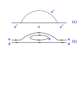
Figure 1: The leading nonanalytic contribution to the chiral expansion of the $\rho$-meson mass. The meson dressing (a) and its associated quark-flow diagram (b) are illustrated.

The two-pion contribution to the $\rho$-meson self-energy is depicted in Fig. 2. This channel gives rise to the next-to-leading nonanalytic (NLNA) contribution to the chiral expansion of the $\rho$-meson mass. Importantly, this contribution also ensures that the $\rho$ develops a finite width as the two-$\pi$ decay becomes accessible.

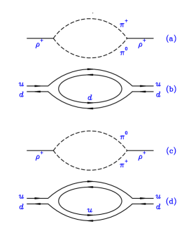
Figure 2: Two-pion contributions to the positively charged $\rho$-meson self-energy. The quark-flow diagrams corresponding to the meson dressings of (a) and (c) are illustrated in (b) and (d) respectively.

As these channels can only come about through the inclusion of a sea-quark loop, the expressions for the pionic self-energies are as given in Ref. adel_rho , but with the pion mass being $M^{non-deg}_{PS}$, corresponding to one valence quark and one sea quark.

In the case of the partially-quenched $\eta^{\prime}$ contributions to the chiral expansion of pQQCD, we simplify the calculation by assuming (as in Ref. Labrenz:1996jy ) that the Witten-Veneziano coupling is simply a constant, $-\mu_{0}^{2}$, and take the limit $\mu_{0}\rightarrow\infty$ after summing all relevant sea quark bubble diagrams. The philosophy is that the physical $\eta^{\prime}$ mass is so large that we can ignore $\eta^{\prime}$ loops in full QCD.

The $\eta^{\prime}$ contributions to the $\rho$-meson self energy are depicted in Fig. 3(a) with the associated quark flow diagrams illustrated in Fig. 3(b) through (f). While Fig. 3(c) appears in quenched QCD, it is complemented by an infinite series of terms, the first few of which are depicted in Fig. 3(d) through (f). Only the sum of Fig. 3(b) through (f) and beyond raise the $\eta^{\prime}$ mass in full QCD.

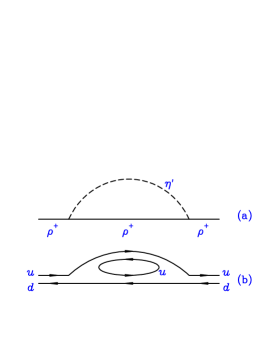
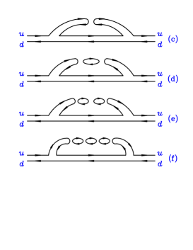
Figure 3: The $\eta^{\prime}$ contribution to the $\rho$-meson self energy and its associated quark flow diagrams in pQQCD. While diagram (c) appears in quenched QCD, it is complemented by an infinite series of terms, the first few of which are depicted in diagrams (d) through (f).

In partially quenched QCD it is essential to track the masses of the pseudoscalar mesons contributing to the quark-flow diagrams of Fig. 3. Whereas Fig. 3(b) involves a non-degenerate pseudoscalar meson, Fig. 3(c) involves degenerate pseudoscalar mesons, and the remaining figures involve both degenerate and non-degenerate pseudoscalar mesons. The sum of diagrams (b) through (f) of Fig. 3 and beyond generate an $\eta^{\prime}$ propagator proportional to

$$\frac{g_{2}^{2}}{q^{2}+{M^{non-deg}_{PS}}^{2}}-\frac{g_{2}^{2}\,\mu_{0}^{2}}{\left(q^{2}+{M^{deg}_{PS}}^{2}\right)^{2}}\left[1-\frac{\mu_{0}^{2}}{q^{2}+{M^{unit}_{PS}}^{2}}+\left(\frac{\mu_{0}^{2}}{q^{2}+{M^{unit}_{PS}}^{2}}\right)^{2}-\cdots\right]\,.$$ (2)

Upon summing the terms in $[\cdots]$, Eq. (2) takes the form

$$\frac{g_{2}^{2}}{q^{2}+{M^{non-deg}_{PS}}^{2}}-g_{2}^{2}\frac{q^{2}+{M^{unit}_{PS}}^{2}}{\left(q^{2}+{M^{deg}_{PS}}^{2}\right)^{2}}\,\frac{\mu_{0}^{2}}{q^{2}+{M^{unit}_{PS}}^{2}+\mu_{0}^{2}}\,.$$ (3)

We note that for equal valence- and sea-quark masses where $M^{deg}_{PS}=M^{non-deg}_{PS}=M^{unit}_{PS}$, Eq. (3) describes the propagation of a heavy $\eta^{\prime}$ meson. Upon taking $\mu_{0}\to\infty$

$$\sigma^{\rm tot}_{\eta^{\prime}\rho}\sim\frac{g_{2}^{2}}{q^{2}+{M^{non-deg}_{PS}}^{2}}-\frac{g_{2}^{2}\left(q^{2}+{M^{unit}_{PS}}^{2}\right)}{\left(q^{2}+{M^{deg}_{PS}}^{2}\right)^{2}}\,,$$ (4)

By subtracting and adding $\left(q^{2}+{M^{deg}_{PS}}^{2}\right)^{-1}$ to the first and second terms respectively, this can be rearranged as

$$\sigma^{\rm tot}_{\eta^{\prime}\rho}\sim\frac{g_{2}^{2}({M^{deg}_{PS}}^{2}-{M^{non-deg}_{PS}}^{2})}{(q^{2}+{M^{non-deg}_{PS}}^{2})(q^{2}+{M^{deg}_{PS}}^{2})}+\frac{g_{2}^{2}({M^{deg}_{PS}}^{2}-{M^{unit}_{PS}}^{2})}{(q^{2}+{M^{deg}_{PS}}^{2})^{2}}$$ (5)

which clearly vanishes when the sea and valence quark masses are equal.

The quenched coupling of a light $\eta^{\prime}$ meson (degenerate with the pion) depicted in Fig. 4(a) is complemented by an infinite sum of sea-quark loop contributions in pQQCD, the first few of which are depicted in Fig. 4(b) through (d). Using similar techniques, one can show that the sum of these graphs leads to the propagation of a heavy $\eta^{\prime}$ and upon taking $\mu_{0}\to\infty$ the contribution of Fig. 4 vanishes.

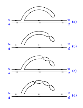
Figure 4: The quenched coupling of a light $\eta^{\prime}$ meson (degenerate with the pion) depicted in (a) is complemented by an infinite sum of sea-quark loop contributions in pQQCD, the first few of which are depicted in (b) through (d).

We note that the coupling $g_{2}$ introduced in Ref. Chow:1997dw , takes the value 0.75, where in terms of the usual $\omega\rho\pi$ coupling constant, $g_{\omega\rho\pi}$ = 16 GeV^-1, $g_{2}^{2}=g_{\omega\rho\pi}^{2}f_{\pi}^{2}/4$. Introducing $f_{\rho\pi\omega}^{2}=\mu_{\rho}g_{2}^{2}$ (with $\mu_{\rho(\pi)}$ the physical $\rho(\pi)$ mass), the total, non-trivial $\eta^{\prime}$ contribution can be written in the form (following Ref. adel_rho for large vector meson mass):

$$\Sigma^{\rho}_{\eta^{\prime}\rho} = \frac{f_{\rho\pi\omega}^{2}}{3\pi^{2}f_{\pi}^{2}}\int_{0}^{\infty}\frac{k^{4}\,u^{2}(k)~{}dk}{(k^{2}+(M_{PS}^{non-deg})^{2})\,(k^{2}+(M_{PS}^{deg})^{2})}\times((M_{PS}^{non-deg})^{2}-(M_{PS}^{deg})^{2})$$ (6)

$$+ \frac{f_{\rho\pi\omega}^{2}}{3\pi^{2}f_{\pi}^{2}}\int_{0}^{\infty}\frac{k^{4}\,u^{2}(k)~{}dk}{(k^{2}+(M_{PS}^{deg})^{2})^{2}}\times((M_{PS}^{unit})^{2}-(M_{PS}^{deg})^{2})\,,$$

In summary, we find

$$\Sigma_{TOT}=\Sigma^{\rho}_{\pi\pi}+\Sigma^{\rho}_{\pi\omega}+\Sigma^{\rho}_{\eta^{\prime}\rho}\,,$$ (7)

where the pion self-energies are given by:

$$\Sigma^{\rho}_{\pi\pi} = -\frac{f_{\rho\pi\pi}^{2}}{6\pi^{2}}\int_{0}^{\infty}\frac{k^{4}\,u_{\pi\pi}^{2}(k)~{}dk}{\omega_{\pi}(k)\,(\omega_{\pi}^{2}(k)-\mu_{\rho}^{2}/4)},$$ (8)

$$\Sigma^{\rho}_{\pi\omega} = -\frac{f_{\rho\pi\omega}^{2}}{3\pi^{2}f_{\pi}^{2}}\int_{0}^{\infty}\frac{k^{4}\,u_{\pi\omega}^{2}(k)~{}dk}{\omega_{\pi}(k)\,(\omega_{\pi}(k)+\Delta M_{\omega\rho})}\,,$$ (9)

and

$$\omega_{\pi}^{2}(k)=k^{2}+(M^{non-deg}_{PS})^{2}\,.$$ (10)

As the $\omega$ meson contributes via a sea-quark loop as illustrated in Fig. 1, the mass splitting between the $\rho$ and $\omega$ is

$$\Delta M_{\omega\rho}=M_{V}^{non-deg}-M_{V}^{deg}\,.$$ (11)

We note that $(\omega_{\pi}(k)+\Delta M_{\omega\rho})>0$ for all quark masses and nontrivial momenta considered in the lattice analysis. We use the values $f_{\rho\pi\pi}=6.028$ (obtained from Ref. adel_rho ) and $f_{\pi}=92.4\,{\rm MeV}$. We use a standard dipole form factor, which takes the form

$$u(k) = \frac{\Lambda^{4}}{(\Lambda^{2}+k^{2})^{2}}\,,$$

$$u_{\pi\omega}(k) = u(k)\,,$$

$$u_{\pi\pi}(k) = u(k)\,u^{-1}(\sqrt{\mu_{\rho}^{2}/4-\mu_{\pi}^{2}})\,,$$

where the second factor in $u_{\pi\pi}(k)$ ensures the correct on-shell normalization condition.

To account for finite volume artefacts, the self-energy equations are discretised so that only those momenta allowed on the lattice appear adel_rho ; Young:2002cj :

$$4\pi\int_{0}^{\infty}k^{2}dk=\int d^{3}k\approx\frac{1}{V}\left(\frac{2\pi}{a}\right)^{3}\sum_{k_{x},k_{y},k_{z}}\,,$$ (12)

with

$$k_{x,y,z}=\frac{2\pi(i,j,k)}{aN_{x,y,z}}\,.$$ (13)

The purpose of the finite-range regulator is to regularise the theory as $k_{x}$, $k_{y}$, $k_{z}$ tend to infinity. Indeed, once any one of $k_{x}$, $k_{y}$ or $k_{z}$ is greater than $\sim 10\Lambda$ the contribution to the integral is negligible and thereby ensuring convergence of the summation. Hence, we would like the highest momentum in each direction to be just over $10\Lambda$. For practical calculation, we therefore use the following to calculate the maxima and minima for i, j, k:

$$(i,j,k)_{max} = ~{}~{}\left[\frac{10\Lambda~{}a}{2\pi}~{}N_{(x,y,z)}\right]+1,$$

$$(i,j,k)_{min} = -\left[\frac{10\Lambda~{}a}{2\pi}~{}N_{(x,y,z)}\right]-1,$$

where $[\ldots]$ denotes the integer part.

We study a range of values of $\Lambda$, starting with the value, $\Lambda_{\pi\omega}=630$ MeV, used in Ref. adel_rho . Figure 5 shows the various self-energy contributions, $\Sigma^{\rho}_{\pi\pi},\Sigma^{\rho}_{\pi\omega}$ and $\Sigma^{\rho}_{\eta^{\prime}\rho}$ as a function of $M_{PS}^{non-deg}$ (see Eqs. (8), (9) and (6) ) for the representative $(\beta,\kappa_{\rm sea})=(2.10,0.1382)$ dataset. In Sec. IV.3 we perform a highly constrained fit to a large “global” dataset, and this enables us to determine a best value of $\Lambda$ which minimises the global $\chi^{2}$.

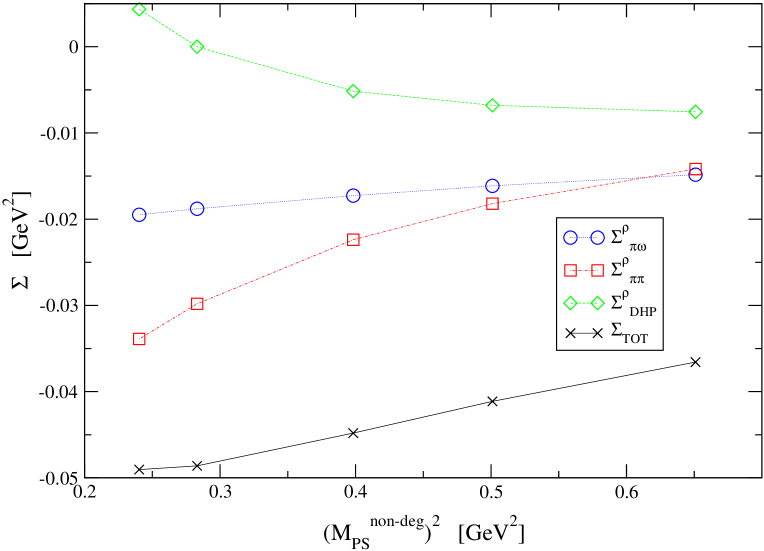
Figure 5: The self-energy contributions (see Eqs. 8, 9 & 6) versus $M_{PS}^{non-deg}$ data for the ensemble $(\beta,\kappa_{\rm sea})=(2.10,0.1382)$ using $\Lambda=630$ MeV.

III Overview of CP-PACS Data

In Ref. cppacs , the CP-PACS collaboration published meson spectrum data from dynamical simulations for mean-field improved Wilson fermions with improved gluons at four different $\beta$ values. For each value of $\beta$, ensembles were generated for four different values of $\kappa_{\rm sea}$ – giving a total of 16 independent ensembles. Table 1 summarises the lattice parameters used. The pseudoscalar- to vector-meson mass ratio $M^{unit}_{PS}/M^{unit}_{V}$ (which gives a measure of the mass of the sea quarks used) varies from 0.55 to 0.80 and the lattice spacing, $a$, from around 0.09 to 0.29 fm. For each of the 16 ensembles there are five $\kappa_{\rm val}$ values considered cppacs . Thus there are a total of 80 $(M_{V}^{deg},M_{PS}^{deg})$ data points available for analysis. In our study we consider the two cases where the lattice spacing is set using either $r_{0}$ sommer or the string tension $\sigma$.

$\beta$	$\kappa_{sea}$	Volume	$M_{PS}^{unit}/M_{V}^{unit}$	$a_{r_{0}}$ [fm]	$a_{\sigma}$ [fm]
1.80	0.1409	$12^{3}\times 24$	0.8067${\scriptstyle{}^{+{9}}_{-{9}}}$	0.286${\scriptstyle{}^{+{6}}_{-{6}}}$	0.288${\scriptstyle{}^{+{3}}_{-{3}}}$
1.80	0.1430	$12^{3}\times 24$	0.7526${\scriptstyle{}^{+{16}}_{-{15}}}$	0.272${\scriptstyle{}^{+{2}}_{-{2}}}$	0.280${\scriptstyle{}^{+{4}}_{-{5}}}$
1.80	0.1445	$12^{3}\times 24$	0.694${\scriptstyle{}^{+{2}}_{-{2}}}$	0.258${\scriptstyle{}^{+{4}}_{-{4}}}$	0.269${\scriptstyle{}^{+{2}}_{-{3}}}$
1.80	0.1464	$12^{3}\times 24$	0.547${\scriptstyle{}^{+{4}}_{-{4}}}$	0.237${\scriptstyle{}^{+{4}}_{-{4}}}$	0.248${\scriptstyle{}^{+{2}}_{-{3}}}$
1.95	0.1375	$16^{3}\times 32$	0.8045${\scriptstyle{}^{+{11}}_{-{11}}}$	0.196${\scriptstyle{}^{+{4}}_{-{4}}}$	0.2044${\scriptstyle{}^{+{10}}_{-{12}}}$
1.95	0.1390	$16^{3}\times 32$	0.752${\scriptstyle{}^{+{2}}_{-{2}}}$	0.185${\scriptstyle{}^{+{3}}_{-{3}}}$	0.1934${\scriptstyle{}^{+{14}}_{-{15}}}$
1.95	0.1400	$16^{3}\times 32$	0.690${\scriptstyle{}^{+{2}}_{-{2}}}$	0.174${\scriptstyle{}^{+{2}}_{-{2}}}$	0.1812${\scriptstyle{}^{+{12}}_{-{12}}}$
1.95	0.1410	$16^{3}\times 32$	0.582${\scriptstyle{}^{+{3}}_{-{3}}}$	0.163${\scriptstyle{}^{+{2}}_{-{2}}}$	0.1699${\scriptstyle{}^{+{13}}_{-{15}}}$
2.10	0.1357	$24^{3}\times 48$	0.806${\scriptstyle{}^{+{2}}_{-{2}}}$	0.1275${\scriptstyle{}^{+{5}}_{-{5}}}$	0.1342${\scriptstyle{}^{+{8}}_{-{8}}}$
2.10	0.1367	$24^{3}\times 48$	0.755${\scriptstyle{}^{+{2}}_{-{2}}}$	0.1203${\scriptstyle{}^{+{4}}_{-{5}}}$	0.1254${\scriptstyle{}^{+{8}}_{-{8}}}$
2.10	0.1374	$24^{3}\times 48$	0.691${\scriptstyle{}^{+{3}}_{-{3}}}$	0.1157${\scriptstyle{}^{+{4}}_{-{4}}}$	0.1203${\scriptstyle{}^{+{6}}_{-{6}}}$
2.10	0.1382	$24^{3}\times 48$	0.576${\scriptstyle{}^{+{3}}_{-{4}}}$	0.1093${\scriptstyle{}^{+{3}}_{-{3}}}$	0.1129${\scriptstyle{}^{+{4}}_{-{5}}}$
2.20	0.1351	$24^{3}\times 48$	0.799${\scriptstyle{}^{+{3}}_{-{3}}}$	0.0997${\scriptstyle{}^{+{4}}_{-{5}}}$	0.10503${\scriptstyle{}^{+{15}}_{-{15}}}$
2.20	0.1358	$24^{3}\times 48$	0.753${\scriptstyle{}^{+{4}}_{-{4}}}$	0.0966${\scriptstyle{}^{+{4}}_{-{4}}}$	0.1013${\scriptstyle{}^{+{3}}_{-{2}}}$
2.20	0.1363	$24^{3}\times 48$	0.705${\scriptstyle{}^{+{6}}_{-{6}}}$	0.0936${\scriptstyle{}^{+{4}}_{-{4}}}$	0.0978${\scriptstyle{}^{+{3}}_{-{3}}}$
2.20	0.1368	$24^{3}\times 48$	0.632${\scriptstyle{}^{+{8}}_{-{8}}}$	0.0906${\scriptstyle{}^{+{4}}_{-{4}}}$	0.0949${\scriptstyle{}^{+{2}}_{-{2}}}$

Table 1: The lattice parameters of the CP-PACS simulation used in this data analysis, taken from Ref. cppacs . The superscript unit refers to the unitary data (i.e., where $\kappa_{\rm val}^{1}\equiv\kappa_{\rm val}^{2}\equiv\kappa_{\rm sea}$). Note that the errors reported in this table are obtained with our bootstrap ensembles (see text).

In the absence of the full set of original CP-PACS data, we generate 1000 bootstrap clusters for all $M_{PS}$ and $M_{V}$ data using a Gaussian distribution whose central value and full width half maximum (FWHM) are the same as the central values and errors published in the Table XXI of Ref. cppacs . Of course, our errors are totally uncorrelated throughout – i.e., each $M_{V}(\beta,\kappa_{\rm sea};\kappa_{\rm val}^{1},\kappa_{\rm val}^{2})$ bootstrap cluster is uncorrelated with the corresponding $M_{PS}(\beta,\kappa_{\rm sea};\kappa_{\rm val}^{1},\kappa_{\rm val}^{2})$ bootstrap cluster. Furthermore, the $M(\beta,\kappa_{\rm sea};\kappa_{\rm val}^{1},\kappa_{\rm val}^{2})$ data is not correlated with the $M(\beta^{\prime},\kappa_{\rm sea}^{\prime};\kappa_{\rm val}^{1},\kappa_{\rm val}^{2})$ data, and nor is the $M(\beta,\kappa_{\rm sea};\kappa_{\rm val}^{1},\kappa_{\rm val}^{2})$ data correlated with that for $M(\beta,\kappa_{\rm sea};\kappa_{\rm val}^{1^{\prime}},\kappa_{\rm val}^{2^{\prime}})$.

We expect therefore that the statistical errors of our final results will be overestimates of the true error, since we have not benefited from the partial cancellation of statistical errors which occurs when combining correlated data. We can obtain a rough estimate of the increase in our errors due to the fact that we don’t maintain correlations as follows. The ratio $M_{PS}^{unit}/M_{V}^{unit}$ listed in Table 1 is obtained from our bootstrap data. Comparing this with the $M_{PS}^{unit}/M_{V}^{unit}$ data in Table XXI of Ref. cppacs (which benefits from the cancellation of correlations), we see that a very rough estimate of the effect of ignoring correlations is to increase the errors by $\sim$20%. We expect that a similar increase in errors will apply to other quantities.

The lattice spacings $a_{r_{0},\sigma}$ were obtained from Table XII of Ref. cppacs using $r_{0}=0.49$ fm and $\sqrt{\sigma}=440$ MeV. Again we generated 1000 bootstrap clusters with a Gaussian distribution, as in the meson mass data. Figure 6 shows the unitary (i.e., $\kappa_{\rm val}^{1}\equiv\kappa_{\rm val}^{2}\equiv\kappa_{\rm sea}$) pseudoscalar mass plotted against the lattice spacing, $a_{r_{0}}$, for the 16 ensembles in Table 1. (Note that $(M_{PS}^{unit})^{2}$ is a direct measure of the sea quark mass since, from PCAC, $(M_{PS}^{unit})^{2}\propto m^{q}_{\rm sea}$.) Also shown for reference are the physical pseudoscalar mesons $\pi,K$ and $``\eta_{s}"$. Note the large range of both the lattice spacing $a_{r_{0}}$ and $m^{q}_{\rm sea}$ in the simulations, and that the lattice spacing is primarily determined by the $\beta$ value, rather than the value of $m^{q}_{\rm sea}$.

The physical volume for these 16 ensembles is $La\approx 2.5$ fm for the $\beta=1.80,1.95$ and $2.10$ cases, but the $\beta=2.20$ ensemble had a slightly smaller physical volume. The associated finite volume effects are incorporated through evaluating the chiral loops by explicitly summing the discrete pion momenta allowed on the lattice. We treat all 16 ensembles on an equal footing. The finite-volume effects are corrected when making contact with the physical observables by evaluating the chiral loop integrals with continuous loop momenta.

The action used in Ref. cppacs is mean-field improved, rather than non-perturbatively improved and will therefore have some residual lattice systematic errors of ${\cal O}(a)$ scaling . We fit the data assuming both ${\cal O}(a)$ and ${\cal O}(a^{2})$ effects in sections IV.2 and IV.3, and are thus able to obtain continuum predictions. Our empirical analysis suggests that nonanalytic terms generated in a dual expansion of both $a$ and $m_{q}$ Bar:2004xp ; Rupak:2002sm ; Bar:2003mh ; Aoki:2003yv ; Beane:2003xv ; Grigoryan:2005zj are either small or can be absorbed at present into the ${\cal O}(a)$ and ${\cal O}(a^{2})$ effects considered here.

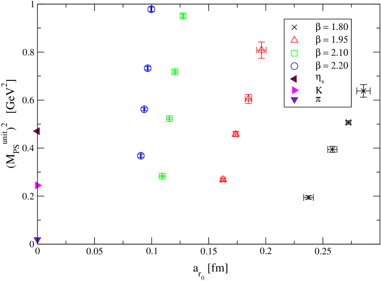
Figure 6: The range of sea quark mass $(M_{PS}^{unit})^{2}$ and lattice spacing, $a_{r_{0}}$, covered by the CP-PACS data displayed in Table 1. $(M_{PS}^{unit})^{2}$ is the pseudoscalar meson mass squared at the unitary point; i.e., where $\kappa_{\rm val}\equiv\kappa_{\rm sea}$. The experimental points for the $\pi,K$ and “$\eta_{s}$” mesons are also shown for reference.

IV Fitting Analysis

IV.1 Summary of Analysis Techniques

Our chiral extrapolation approach is based upon converting all masses into physical units prior to any extrapolation being performed. An alternative approach would be to extrapolate dimensionless masses (in lattice units) cppacs . However, using physical units offers the following key advantages:

• The data from different ensembles can be combined in a global fit. If the masses were left in dimensionless units, there would be no possibility of combining data at different lattice spacings together into such a global fit.

• Dimensionful mass predictions from lattice simulations are effectively mass ratios, and hence one would expect some of the systematic (and statistical) errors to cancel. That is, $M^{dimful}=M^{\#}\times a^{-1}\equiv M^{\#}/M_{\Omega}^{\#}\times M_{\Omega}^{expt}$, where $\Omega$ is the quantity used to set the lattice spacing, $a$, the superscripts #, $expt$ refer to the lattice mass estimate and the experimental value, respectively.

• Lattice data are not in the regime where the coefficients of nonanalytic terms in the chiral expansion can be reliably constrained. These dimensionful quantities must therefore be fixed to their phenomenological values.

In this paper we use two different quantities for setting the scale, $r_{0}$ and $\sigma$ – although we have a preference, as explained in Sec. IV.3, for $r_{0}$. Table 1 lists values for $a_{r_{0}}$ and $a_{\sigma}$.

In our chiral extrapolations we use two basic fitting functions, the finite-range regularisation method (hereafter referred to as the “Adelaide” method)

$$\sqrt{(M_{V}^{deg})^{2}-\Sigma_{TOT}} = a_{0}+a_{2}(M_{PS}^{deg})^{2}+a_{4}(M_{PS}^{deg})^{4}+a_{6}(M_{PS}^{deg})^{6},$$ (14)

where $\Sigma_{TOT}$ is calculated using Eq. (7), and a naive polynomial fit

$$M_{V}^{deg}=a_{0}+a_{2}(M_{PS}^{deg})^{2}+a_{4}(M_{PS}^{deg})^{4}+a_{6}(M_{PS}^{deg})^{6}.$$ (15)

In each case we refer to these fits as “cubic” since they include cubic terms in the chiral expansion of $m_{q}\propto(M_{PS})^{2}$. We also perform fits with the coefficient $a_{6}$ set to zero in Eqs.(14) and (15), referring to these as “quadratic”. It is worth noting that the dominant functional form of $M_{V}$ with $(M_{PS}^{deg})^{2}$ is linear (see, for example, Fig. 7, where the LHS of Eqs. (14) and (15) are referred to as $M_{V}^{\rm sub}$). We exploit this fact in the fitting functions given above. In particular, this is why the Adelaide fit uses $\sqrt{(M_{V}^{deg})^{2}-\Sigma_{TOT}}$ on the LHS rather than $(M_{V}^{deg})^{2}-\Sigma_{TOT}$ which would, a priori, be an equally valid chiral expansion. Thus, with the above functional forms, we expect the coefficients, $a_{n}$, to be small for $n\geq 4$ and this is, in fact, what we find.

In the following, we first use Eqs. (14) and (15) to fit the 16 ensembles in Table 1 separately. We then turn to a global fit, where all 16 ensembles are combined in one fitting function.

IV.2 Individual ensemble fits

We begin our analysis by fitting the meson spectrum of each of the 16 ensembles listed in Table 1 separately. In this section we use $r_{0}$ to set the scale and select a value of $\Lambda=650$ MeV (see Sec. IV.3). We use both the Adelaide, Eq. (14), and naive, Eq. (15), fitting functions and restrict our attention to quadratic ($a_{6}\equiv 0$) chiral fits, since there are only five $(M_{V}^{deg},M_{PS}^{deg})$ data points available for each ensemble. The coefficients, $a_{0,2,4}$, obtained by fitting $M_{V}$ against $M_{PS}$ with both the naive (Eq. (15)) and Adelaide (Eq. (14)) fitting functions are listed in Table 2. We see that the $a_{4}$ coefficients are both small and generally poorly determined, confirming our decision to fit to the quadratic, rather than the cubic, chiral extrapolation form. We note also that there is some agreement between the naive and Adelaide $a_{0,2}$ coefficients, although their variation with $\kappa_{\rm sea}$ tends to be different.

$\beta$	$\kappa_{sea}$	$a^{naive}_{0}$	$a^{adel}_{0}$	$a^{naive}_{2}$	$a^{adel}_{2}$	$a^{naive}_{4}$	$a^{adel}_{4}$
		[GeV]	[GeV]	[GeV-1]	[GeV-1]	[GeV-3]	[GeV-3]
1.80	0.1409	0.701${\scriptstyle{}^{+{14}}_{-{22}}}$	0.70${\scriptstyle{}^{+{2}}_{-{2}}}$	0.46${\scriptstyle{}^{+{7}}_{-{3}}}$	0.54${\scriptstyle{}^{+{5}}_{-{5}}}$	-0.01${\scriptstyle{}^{+{3}}_{-{7}}}$	-0.09${\scriptstyle{}^{+{5}}_{-{5}}}$
1.80	0.1430	0.712${\scriptstyle{}^{+{14}}_{-{13}}}$	0.724${\scriptstyle{}^{+{14}}_{-{13}}}$	0.48${\scriptstyle{}^{+{6}}_{-{6}}}$	0.51${\scriptstyle{}^{+{5}}_{-{6}}}$	-0.04${\scriptstyle{}^{+{6}}_{-{6}}}$	-0.08${\scriptstyle{}^{+{6}}_{-{6}}}$
1.80	0.1445	0.73${\scriptstyle{}^{+{2}}_{-{2}}}$	0.756${\scriptstyle{}^{+{14}}_{-{15}}}$	0.43${\scriptstyle{}^{+{5}}_{-{5}}}$	0.44${\scriptstyle{}^{+{5}}_{-{5}}}$	0.01${\scriptstyle{}^{+{5}}_{-{5}}}$	-0.01${\scriptstyle{}^{+{5}}_{-{5}}}$
1.80	0.1464	0.72${\scriptstyle{}^{+{2}}_{-{2}}}$	0.769${\scriptstyle{}^{+{13}}_{-{15}}}$	0.49${\scriptstyle{}^{+{5}}_{-{5}}}$	0.43${\scriptstyle{}^{+{5}}_{-{5}}}$	-0.02${\scriptstyle{}^{+{6}}_{-{6}}}$	0.007${\scriptstyle{}^{+{59}}_{-{58}}}$
1.95	0.1375	0.76${\scriptstyle{}^{+{2}}_{-{2}}}$	0.75${\scriptstyle{}^{+{2}}_{-{2}}}$	0.49${\scriptstyle{}^{+{4}}_{-{4}}}$	0.53${\scriptstyle{}^{+{4}}_{-{4}}}$	-0.05${\scriptstyle{}^{+{4}}_{-{3}}}$	-0.08${\scriptstyle{}^{+{3}}_{-{3}}}$
1.95	0.1390	0.76${\scriptstyle{}^{+{2}}_{-{2}}}$	0.772${\scriptstyle{}^{+{17}}_{-{15}}}$	0.47${\scriptstyle{}^{+{4}}_{-{4}}}$	0.49${\scriptstyle{}^{+{4}}_{-{4}}}$	-0.03${\scriptstyle{}^{+{4}}_{-{3}}}$	-0.05${\scriptstyle{}^{+{4}}_{-{4}}}$
1.95	0.1400	0.785${\scriptstyle{}^{+{12}}_{-{12}}}$	0.803${\scriptstyle{}^{+{11}}_{-{11}}}$	0.43${\scriptstyle{}^{+{4}}_{-{4}}}$	0.44${\scriptstyle{}^{+{4}}_{-{4}}}$	-0.01${\scriptstyle{}^{+{3}}_{-{3}}}$	-0.02${\scriptstyle{}^{+{3}}_{-{3}}}$
1.95	0.1410	0.766${\scriptstyle{}^{+{13}}_{-{15}}}$	0.799${\scriptstyle{}^{+{13}}_{-{14}}}$	0.48${\scriptstyle{}^{+{5}}_{-{4}}}$	0.45${\scriptstyle{}^{+{5}}_{-{4}}}$	-0.03${\scriptstyle{}^{+{4}}_{-{4}}}$	-0.03${\scriptstyle{}^{+{3}}_{-{4}}}$
2.10	0.1357	0.829${\scriptstyle{}^{+{14}}_{-{14}}}$	0.820${\scriptstyle{}^{+{14}}_{-{14}}}$	0.42${\scriptstyle{}^{+{5}}_{-{4}}}$	0.46${\scriptstyle{}^{+{5}}_{-{4}}}$	-0.02${\scriptstyle{}^{+{3}}_{-{4}}}$	-0.05${\scriptstyle{}^{+{3}}_{-{4}}}$
2.10	0.1367	0.794${\scriptstyle{}^{+{11}}_{-{10}}}$	0.797${\scriptstyle{}^{+{11}}_{-{10}}}$	0.50${\scriptstyle{}^{+{3}}_{-{3}}}$	0.53${\scriptstyle{}^{+{3}}_{-{3}}}$	-0.06${\scriptstyle{}^{+{3}}_{-{3}}}$	-0.08${\scriptstyle{}^{+{3}}_{-{2}}}$
2.10	0.1374	0.807${\scriptstyle{}^{+{13}}_{-{14}}}$	0.822${\scriptstyle{}^{+{13}}_{-{14}}}$	0.48${\scriptstyle{}^{+{4}}_{-{4}}}$	0.49${\scriptstyle{}^{+{4}}_{-{4}}}$	-0.05${\scriptstyle{}^{+{3}}_{-{3}}}$	-0.06${\scriptstyle{}^{+{3}}_{-{3}}}$
2.10	0.1382	0.781${\scriptstyle{}^{+{10}}_{-{9}}}$	0.814${\scriptstyle{}^{+{10}}_{-{9}}}$	0.53${\scriptstyle{}^{+{3}}_{-{3}}}$	0.50${\scriptstyle{}^{+{3}}_{-{3}}}$	-0.08${\scriptstyle{}^{+{2}}_{-{2}}}$	-0.07${\scriptstyle{}^{+{2}}_{-{2}}}$
2.20	0.1351	0.84${\scriptstyle{}^{+{3}}_{-{3}}}$	0.84${\scriptstyle{}^{+{3}}_{-{3}}}$	0.43${\scriptstyle{}^{+{8}}_{-{8}}}$	0.46${\scriptstyle{}^{+{8}}_{-{8}}}$	-0.02${\scriptstyle{}^{+{6}}_{-{6}}}$	-0.04${\scriptstyle{}^{+{6}}_{-{6}}}$
2.20	0.1358	0.83${\scriptstyle{}^{+{2}}_{-{2}}}$	0.84${\scriptstyle{}^{+{2}}_{-{2}}}$	0.44${\scriptstyle{}^{+{7}}_{-{7}}}$	0.46${\scriptstyle{}^{+{7}}_{-{7}}}$	-0.03${\scriptstyle{}^{+{5}}_{-{5}}}$	-0.05${\scriptstyle{}^{+{5}}_{-{5}}}$
2.20	0.1363	0.80${\scriptstyle{}^{+{3}}_{-{3}}}$	0.81${\scriptstyle{}^{+{3}}_{-{3}}}$	0.51${\scriptstyle{}^{+{8}}_{-{8}}}$	0.52${\scriptstyle{}^{+{8}}_{-{8}}}$	-0.07${\scriptstyle{}^{+{6}}_{-{6}}}$	-0.08${\scriptstyle{}^{+{6}}_{-{6}}}$
2.20	0.1368	0.78${\scriptstyle{}^{+{2}}_{-{2}}}$	0.80${\scriptstyle{}^{+{2}}_{-{2}}}$	0.52${\scriptstyle{}^{+{8}}_{-{8}}}$	0.51${\scriptstyle{}^{+{7}}_{-{8}}}$	-0.06${\scriptstyle{}^{+{6}}_{-{6}}}$	-0.06${\scriptstyle{}^{+{6}}_{-{6}}}$

Table 2: The coefficients obtained from fitting $M_{V}$ data against $M_{PS}^{2}$ using both the naive and Adelaide fits (i.e., Eqs. (15) and (14), respectively) for each of the 16 ensembles listed in Table 1. As discussed in the text we restrict these fits to quadratic rather than cubic chiral functions (i.e., $a_{6}\equiv 0$). The scale was set using $r_{0}$.

Figure 7 shows the results of these fits for the $(\beta,\kappa_{\rm sea})=(2.10,0.1382)$ ensemble, which is a good representative of all of them. The scale is set from $r_{0}$, which is our preferred method (see Sec. IV.3). Note that this ensemble’s $(a,m^{q}_{\rm sea})$ coordinates are closest to the physical point $(a,m^{q}_{\rm sea})=(0,m_{u,d})$ for those ensembles with $La\approx 2.5\,$fm – see Fig. 6.

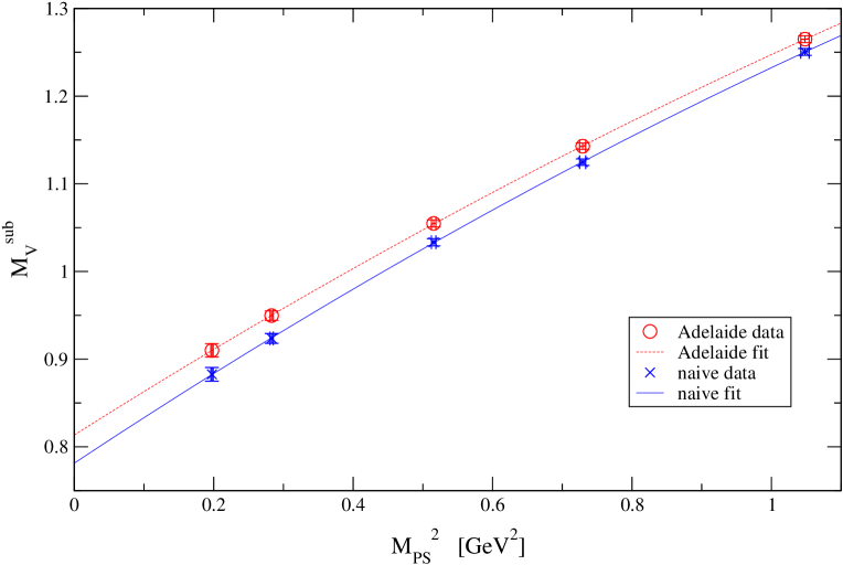
Figure 7: A plot of $M_{V}^{Sub}$ versus $M_{PS}$ data for the ensemble $(\beta,\kappa_{\rm sea})=(2.10,0.1382)$ together with the results of the quadratic Adelaide, Eq. (14), and naive, Eq. (15), fits. $M_{V}^{Sub}$ is defined as $M_{V}^{Sub}=\sqrt{(M_{V}^{deg})^{2}-\Sigma_{TOT}}$ for the Adelaide fit (i.e., the LHS of Eq. 14 - note that $\Sigma_{TOT}$ is negative), and $M_{V}^{Sub}=M_{V}^{deg}$ for the naive fit (i.e., the LHS of Eq. (15)).

The values of $a_{0,2}$ in Table 2 hint at a systematic variation of $a_{0,2}$ with $a_{r_{0}}$. To check this we plot $a_{0}$ and $a_{2}$ against $a_{r_{0}}$ (for both the linear and Adelaide fits) in Figs. 8 and 9. This motivates a continuum extrapolation of the form

$$a_{0,2}=a_{0,2}^{cont}+X^{individual}_{0,2}\;a_{r_{0}}\,.$$ (16)

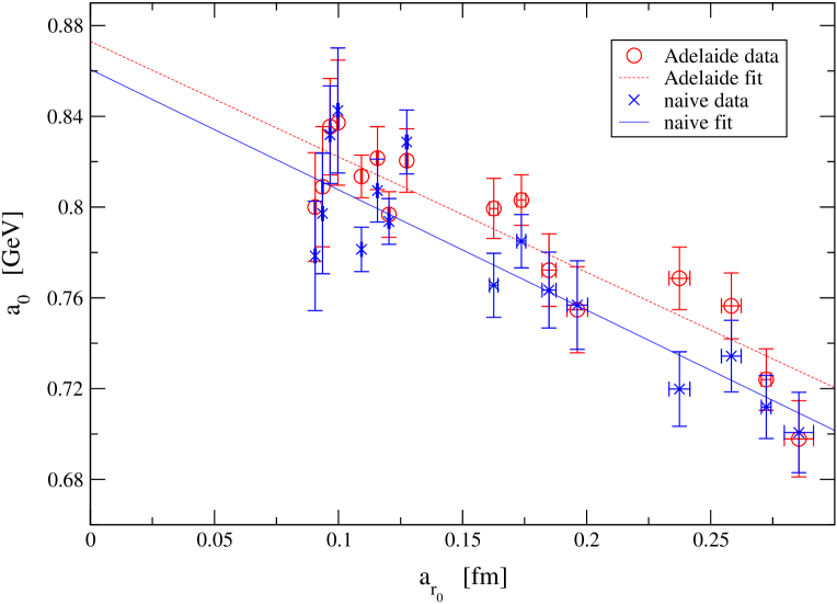
Figure 8: A continuum extrapolation of the $a_{0}$ coefficient obtained from both the Adelaide and naive fits using Eq. (16).

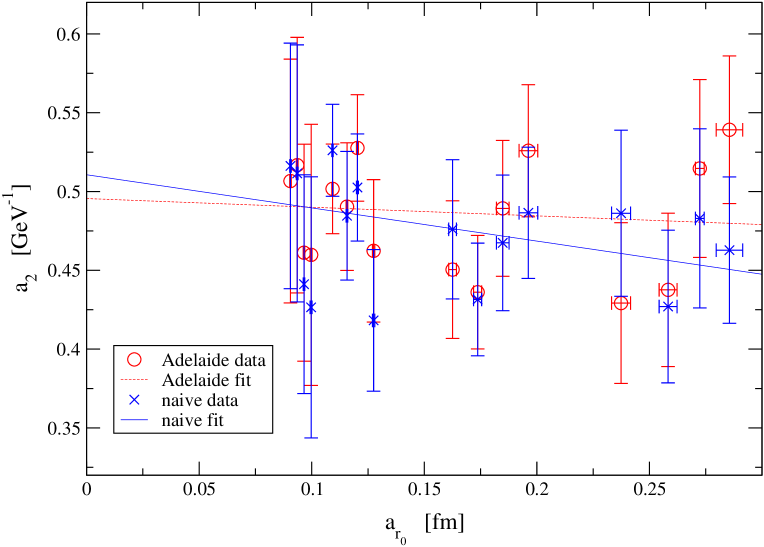
Figure 9: A continuum extrapolation of the $a_{2}$ coefficient obtained from both the Adelaide and naive fits using Eq. (16).

The results of these fits are displayed in Table 3. From the values of $X^{individual}_{0,2}$ in Table 3, we can confirm statistically significant ${\cal O}(a)$ effects in $a_{0}$ but not in $a_{2}$. This will be important in determining our fit procedure in Sec. IV.3.

	$a_{0}^{cont.}$	$X^{individual}_{0}$	$\chi^{2}_{0}/d.o.f.$	$a_{2}^{cont.}$	$X^{individual}_{2}$	$\chi^{2}_{2}/d.o.f.$
	[GeV]	[GeV/fm]		[GeV-1]	[GeV-1/fm]
Naive-fit	0.861${\scriptstyle{}^{+{11}}_{-{9}}}$	-0.53${\scriptstyle{}^{+{5}}_{-{7}}}$	21 / 14	0.51${\scriptstyle{}^{+{3}}_{-{4}}}$	-0.21${\scriptstyle{}^{+{23}}_{-{15}}}$	8 / 14
Adelaide-fit	0.873${\scriptstyle{}^{+{10}}_{-{10}}}$	-0.51${\scriptstyle{}^{+{5}}_{-{6}}}$	16 / 14	0.50${\scriptstyle{}^{+{3}}_{-{3}}}$	-0.06${\scriptstyle{}^{+{19}}_{-{18}}}$	10 / 14

Table 3: The coefficients obtained from the continuum extrapolation of both the naive and Adelaide fits, using the values of $a_{0,2}$ given in Table 2 with Eq. (16).

IV.3 Global fits

We now turn our attention to an analysis of the whole (degenerate) data set. Figure 10 shows all of the degenerate CP-PACS data with the physical scale set using $r_{0}$. Since there are 16 ensembles with five $(M_{V}^{deg},M_{PS}^{deg})$ values in each (see Sec. III), this global fit contains 80 data points. We expect that this large number of data points should produce a highly constrained set of fit parameters, $a_{0,2,\ldots}$.

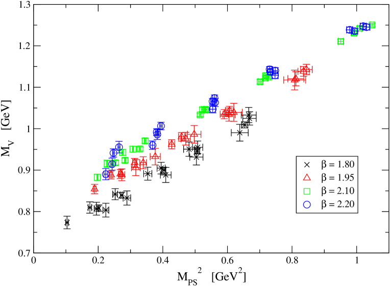
Figure 10: Illustration of the 80 lattice data points of the degenerate CP-PACS data set, with the physical scale of a${}_{r_{0}}$.

Referring to the coefficients listed in Table 2 and the discussion in the previous section, we observe a significant variation amongst the $a_{0}$ values with lattice spacing, whereas the values of $a_{2}$ are approximately constant with lattice spacing. We also recall that the $a_{4}$ coefficient was undetermined. This suggests that we should allow for some variation of the $a_{0}$ coefficient with lattice spacing and in consequence we adopt the following modified version of the Adelaide and naive fitting functions, based on Eqs. (14) and (15).

$$\sqrt{(M_{V}^{deg})^{2}-\Sigma_{TOT}}=(a_{0}^{cont}+X_{1}a+X_{2}a^{2})+a_{2}(M_{PS}^{deg})^{2}+a_{4}(M_{PS}^{deg})^{4}+a_{6}(M_{PS}^{deg})^{6},$$ (17)

and

$$M_{V}^{deg}=(a_{0}^{cont}+X_{1}a+X_{2}a^{2})+a_{2}(M_{PS}^{deg})^{2}+a_{4}(M_{PS}^{deg})^{4}+a_{6}(M_{PS}^{deg})^{6}\,,$$ (18)

respectively. As in the previous section we refer to the above fits as “cubic”, since they include the $a_{6}$ term (which is proportional to $m_{q}^{3}$). As above we also perform fits with $a_{6}$ set to zero, referring to these as “quadratic”. These fitting functions, Eqs. (17) and (18), have both ${\cal O}(a)$ and ${\cal O}(a^{2})$ terms, because the lattice action used is only mean-field improved and will contain ${\cal O}(a^{2})$ errors, together with some residual errors at ${\cal O}(a)$. In the following we will experiment by turning off the ${\cal O}(a)$ term (i.e. by setting $X_{1}\equiv 0$) in Eqs. (17) and (18) in order to see whether these residual ${\cal O}(a)$ errors are significant. Note that we also included ${\cal O}(a,a^{2})$ terms in $a_{2}$ (and even $a_{4}$) as a check but found that these fits were unstable, confirming the findings of the previous section that there are discernible lattice spacing effects only in the $a_{0}$ coefficient.

The global fits used both $r_{0}$ and the string tension, $\sigma$, to set the scale. Thus we have a large number of fit types which are summarised in Table 4. Indeed, there are two choices from each of the four columns in Table 4, making a total of $2^{4}$ fitting procedures. In the following all $2^{4}$ fits were performed.

Approach	Chiral Extrapolation	Treatment of Lattice	Lattice Spacing
		Spacing Artefacts in $a_{0}$	set from
Adelaide	Cubic	$a_{0}$ term has	$r_{0}$
i.e. eq.17	i.e. ${\cal O}(M_{PS}^{6})$ included	${\cal O}(a+a^{2})$ corrections
Naive	Quadratic	$a_{0}$ term has	$\sigma$
i.e. eq.18	i.e. no ${\cal O}(M_{PS}^{6})$ term	only ${\cal O}(a^{2})$ corrections

Table 4: The different fit types used in the global analysis. Fits for each of the $2^{4}$ choices depicted above were performed.

As noted above, the global fits contain 80 data points, and the largest number of fitting parameters is six ($a_{0}^{cont},X_{1},X_{2},a_{2},a_{4}$ and $a_{6}$). Thus the global fits are highly constrained.

Before presenting results from the global fits, we recall our discussion of the $\Lambda$ parameter in Sec. II. The Adelaide approach motivates the introduction of the mass scale, $\Lambda$, as corresponding to the physical size of the pion source in the hadron which controls the chiral physics. It serves to separate the region where chiral physics is important from that where the internal structure of the hadron, which is not part of the effective field theory, becomes dominant. Since we are performing a highly constrained fit procedure, we are able to derive the best $\Lambda$ value from the data as follows. Figure 11 shows the $\chi^{2}/d.o.f.$ as a function of $\Lambda$ and we see that for the results where $r_{0}$ was used to set the scale, all four fitting types display near identical $\chi^{2}$ behaviour, with a distinct minimum at $\Lambda\approx 650$ MeV. In other words, the $\chi^{2}$ behaviour is independent of whether we chirally expand to ${\cal O}(M_{PS}^{4})$ or ${\cal O}(M_{PS}^{6})$ or whether we allow for lattice systematics in the $a_{0}$ coefficient of ${\cal O}(a+a^{2})$ or ${\cal O}(a^{2})$.

For the case where $\sigma$ is used to set the scale, Fig. 11 shows that there is a distinct minimum at $\Lambda\approx 550$ MeV for all four fitting types. All other things being equal, there is no preference between the cubic or quadratic chiral fits. However, the plot clearly shows that the ${\cal O}(a+a^{2})$ fits are favoured, in that they produce a lower $\chi^{2}$ value than the pure ${\cal O}(a^{2})$ fits. As a test, we have also fitted the data with a pure ${\cal O}(a)$ correction (i.e., Eq. (17) with $X_{2}=0$) and found that the $\chi^{2}$ values for this fit overlay those from the ${\cal O}(a+a^{2})$ fits. This is strongly suggestive that the dominant lattice-spacing systematic is ${\cal O}(a)$ when the string tension is used to set the scale.

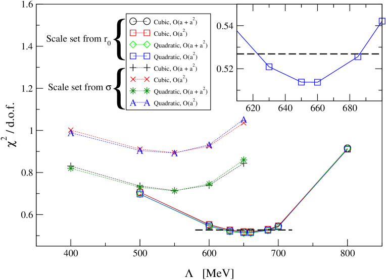
Figure 11: Variation of the $\chi^{2}/d.o.f$ against $\Lambda$. The insert shows a closeup of the minimum for the quadratic fit with ${\cal O}(a^{2})$ errors using $r_{0}$ to set the scale (i.e. the preferred fitting procedure). The dashed horizontal line represents an increase of $\chi^{2}$ from its minimum value by unity for this fit procedure (i.e. it represents one standard deviation) – see Sec. V. The intercept of this dashed line with the $\chi^{2}$ curves (at $\Lambda=$620 and 690 MeV) is used to derive the range of acceptable $\Lambda$ values.

We now use these values of $\Lambda$ (550 MeV and 650 MeV for the $\sigma$ and $r_{0}$ cases, respectively) to perform the 16 global fits discussed above and listed in Table 4. Table 5 gives the coefficients and the $\chi^{2}/d.o.f.$ for each fit.

Fit	Scale	$a_{0}^{cont}$	$X_{1}$	$X_{2}$	$a_{2}$	$a_{4}$	$a_{6}$	$\chi^{2}/d.o.f.$
Approach	from	[GeV]	[GeVfm-1]	[GeVfm-2]	[GeV-1]	[GeV-3]	[GeV-5]
Cubic chiral extrapolation; $a_{0}$ contains ${\cal O}(a+a^{2})$
Adelaide	$r_{0}$	0.844${\scriptstyle{}^{+{13}}_{-{16}}}$	-0.11${\scriptstyle{}^{+{15}}_{-{13}}}$	-1.1${\scriptstyle{}^{+{3}}_{-{4}}}$	0.47${\scriptstyle{}^{+{5}}_{-{4}}}$	-0.02${\scriptstyle{}^{+{8}}_{-{10}}}$	-0.02${\scriptstyle{}^{+{5}}_{-{4}}}$	38 / 74
Adelaide	$\sigma$	0.836${\scriptstyle{}^{+{9}}_{-{11}}}$	-0.37${\scriptstyle{}^{+{10}}_{-{9}}}$	-0.2${\scriptstyle{}^{+{2}}_{-{3}}}$	0.44${\scriptstyle{}^{+{5}}_{-{4}}}$	0.04${\scriptstyle{}^{+{7}}_{-{9}}}$	-0.06${\scriptstyle{}^{+{5}}_{-{4}}}$	53 / 74
Naive	$r_{0}$	0.819${\scriptstyle{}^{+{13}}_{-{17}}}$	-0.15${\scriptstyle{}^{+{15}}_{-{13}}}$	-1.1${\scriptstyle{}^{+{3}}_{-{4}}}$	0.56${\scriptstyle{}^{+{6}}_{-{5}}}$	-0.16${\scriptstyle{}^{+{8}}_{-{10}}}$	0.05${\scriptstyle{}^{+{5}}_{-{4}}}$	77 / 74
Naive	$\sigma$	0.805${\scriptstyle{}^{+{10}}_{-{12}}}$	-0.38${\scriptstyle{}^{+{11}}_{-{9}}}$	-0.3${\scriptstyle{}^{+{2}}_{-{3}}}$	0.57${\scriptstyle{}^{+{5}}_{-{4}}}$	-0.18${\scriptstyle{}^{+{8}}_{-{10}}}$	0.06${\scriptstyle{}^{+{6}}_{-{5}}}$	73 / 74
Cubic chiral extrapolation; $a_{0}$ contains ${\cal O}(a^{2})$ only
Adelaide	$r_{0}$	0.835${\scriptstyle{}^{+{8}}_{-{9}}}$	—	-1.40${\scriptstyle{}^{+{3}}_{-{4}}}$	0.48${\scriptstyle{}^{+{5}}_{-{4}}}$	-0.03${\scriptstyle{}^{+{8}}_{-{10}}}$	-0.02${\scriptstyle{}^{+{5}}_{-{4}}}$	39 / 75
Adelaide	$\sigma$	0.807${\scriptstyle{}^{+{6}}_{-{8}}}$	—	-1.24${\scriptstyle{}^{+{3}}_{-{3}}}$	0.43${\scriptstyle{}^{+{5}}_{-{4}}}$	0.06${\scriptstyle{}^{+{8}}_{-{9}}}$	-0.06${\scriptstyle{}^{+{5}}_{-{4}}}$	67 / 75
Naive	$r_{0}$	0.806${\scriptstyle{}^{+{8}}_{-{10}}}$	—	-1.49${\scriptstyle{}^{+{4}}_{-{4}}}$	0.56${\scriptstyle{}^{+{6}}_{-{5}}}$	-0.17${\scriptstyle{}^{+{8}}_{-{10}}}$	0.06${\scriptstyle{}^{+{5}}_{-{4}}}$	78 / 75
Naive	$\sigma$	0.775${\scriptstyle{}^{+{7}}_{-{8}}}$	—	-1.31${\scriptstyle{}^{+{4}}_{-{4}}}$	0.56${\scriptstyle{}^{+{5}}_{-{4}}}$	-0.16${\scriptstyle{}^{+{8}}_{-{10}}}$	0.05${\scriptstyle{}^{+{5}}_{-{5}}}$	87 / 75
Quadratic chiral extrapolation; $a_{0}$ contains ${\cal O}(a+a^{2})$
Adelaide	$r_{0}$	0.840${\scriptstyle{}^{+{10}}_{-{12}}}$	-0.11${\scriptstyle{}^{+{14}}_{-{13}}}$	-1.1${\scriptstyle{}^{+{3}}_{-{4}}}$	0.493${\scriptstyle{}^{+{12}}_{-{11}}}$	-0.061${\scriptstyle{}^{+{8}}_{-{9}}}$	—	38 / 75
Adelaide	$\sigma$	0.829${\scriptstyle{}^{+{8}}_{-{9}}}$	-0.37${\scriptstyle{}^{+{10}}_{-{9}}}$	-0.2${\scriptstyle{}^{+{2}}_{-{3}}}$	0.490${\scriptstyle{}^{+{13}}_{-{11}}}$	-0.052${\scriptstyle{}^{+{10}}_{-{11}}}$	—	54 / 75
Naive	$r_{0}$	0.828${\scriptstyle{}^{+{11}}_{-{13}}}$	-0.16${\scriptstyle{}^{+{15}}_{-{13}}}$	-1.1${\scriptstyle{}^{+{3}}_{-{4}}}$	0.505${\scriptstyle{}^{+{13}}_{-{11}}}$	-0.068${\scriptstyle{}^{+{9}}_{-{10}}}$	—	78 / 75
Naive	$\sigma$	0.812${\scriptstyle{}^{+{8}}_{-{9}}}$	-0.37${\scriptstyle{}^{+{11}}_{-{9}}}$	-0.3${\scriptstyle{}^{+{2}}_{-{3}}}$	0.523${\scriptstyle{}^{+{13}}_{-{12}}}$	-0.075${\scriptstyle{}^{+{11}}_{-{11}}}$	—	74 / 75
Quadratic chiral extrapolation; $a_{0}$ contains ${\cal O}(a^{2})$ only
Adelaide	$r_{0}$	0.832${\scriptstyle{}^{+{4}}_{-{4}}}$	—	-1.40${\scriptstyle{}^{+{3}}_{-{4}}}$	0.494${\scriptstyle{}^{+{12}}_{-{11}}}$	-0.061${\scriptstyle{}^{+{8}}_{-{9}}}$	—	39 / 76
Adelaide	$\sigma$	0.799${\scriptstyle{}^{+{3}}_{-{4}}}$	—	-1.23${\scriptstyle{}^{+{3}}_{-{3}}}$	0.486${\scriptstyle{}^{+{13}}_{-{11}}}$	-0.046${\scriptstyle{}^{+{10}}_{-{11}}}$	—	68 / 76
Naive	$r_{0}$	0.815${\scriptstyle{}^{+{4}}_{-{4}}}$	—	-1.49${\scriptstyle{}^{+{4}}_{-{4}}}$	0.506${\scriptstyle{}^{+{12}}_{-{11}}}$	-0.068${\scriptstyle{}^{+{8}}_{-{10}}}$	—	79 / 76
Naive	$\sigma$	0.781${\scriptstyle{}^{+{3}}_{-{4}}}$	—	-1.31${\scriptstyle{}^{+{3}}_{-{4}}}$	0.520${\scriptstyle{}^{+{13}}_{-{12}}}$	-0.069${\scriptstyle{}^{+{11}}_{-{11}}}$	—	88 / 76

Table 5: The results of the global fit analysis. Fits for all $2^{4}$ combinations depicted in Table 4 are shown.

Summarising the results of Table 5 and Fig. 11 (and referring to the $2^{4}$ different fit types listed in Table 4) we note:

Fit Approach: The Adelaide method always gives a smaller $\chi^{2}$ than the naive approach, confirming it as the preferred chiral extrapolation procedure.

Chiral Extrapolation: The cubic chiral extrapolation (i.e., introducing the ${\cal O}(M_{PS}^{6})$ term in Eqs. (17) and (18) ) leads to a poorly determined $a_{6}$ coefficient in all cases. Furthermore it causes the $a_{4}$ coefficient to become much more poorly determined than it is in the quadratic chiral extrapolation cases.

Treatment of Lattice Spacing Artefacts in $a_{0}$: From Table 5, when the scale is set from $r_{0}$, the $a_{0}$ and $a_{2}$ coefficients (which are the dominant terms in the chiral extrapolation) do not depend on whether ${\cal O}(a+a^{2})$ or ${\cal O}(a^{2})$–only corrections are applied to the $a_{0}$ coefficient. Indeed, when ${\cal O}(a^{2})$ only corrections are used, the error in $a_{0}$ is reduced. However, when the scale is set from $\sigma$, $a_{0}$ does depend on how the ${\cal O}(a)$ systematics are treated. Note also that $X_{1}$ (i.e. the ${\cal O}(a)$ coefficient) in the $\sigma$ fits are 2–3 times larger than those from the $r_{0}$ fits. This supports our earlier comments above regarding the probable ${\cal O}(a)$ systematics when the $\sigma$ scale was used.

Quantity used to set Lattice Spacing: In the Adelaide approach, setting the scale from $r_{0}$ gives a significantly smaller $\chi^{2}$ than using $\sigma$ (see Fig. 11). Given this, and the comments above regarding the probable ${\cal O}(a)$ systematics in the $\sigma$ data, we use $r_{0}$ as our preferred method for setting the scale. In the naive case the data does not favour setting the scale from either $r_{0}$ or $\sigma$.

On the basis of these results, we choose the quadratic chiral extrapolation method with the scale set from $r_{0}$ and ${\cal O}(a^{2})$ corrections in the $a_{0}$ coefficient to define the central value of both the Adelaide and naive fitting procedure. The spread from the other fitting types is used to define the error. In Sec. V, we determine the predictions for physical $\rho-$meson mass from these fitting types.

V Physical Predictions

We are now ready to estimate $M_{\rho}$ in the continuum using the Adelaide and naive fits performed in the previous section. We obtain this prediction from Eqs. (14) and (15) by setting $M_{PS}^{deg}=M_{PS}^{non-deg}=M_{PS}^{unit}=\mu_{\pi}$. We set $\Delta M_{\omega\rho}$ to zero in this calculation and also note that $\Sigma^{\rho}_{\eta^{\prime}\rho}$ vanishes, as required. Since we are predicting the continuum value for the vector meson mass, we calculate the integrals in Eqs. (8) and (9) directly, rather than using the lattice interpretation of the integral in Eq. (12).

We obtain continuum estimates of all $2^{4}$ fitting types (see Table 4) using the coefficients, $a_{0}^{cont}$ and $a_{2,4,6}$, of the global fits of Sec. IV.3 (i.e., those in Table 5). Table 6 displays these mass predictions. For the Adelaide case we use $\Lambda=650(550)$ MeV, with the physical scale set using $r_{0}(\sigma)$ (see Sec. IV.3). Note that we use the global analysis (Sec. IV.3), rather than the analysis of Sec. IV.2, which treated the ensembles separately, since the global fit is much more tightly constrained.

It is interesting to study the variation in the prediction of the physical mass of the $\rho$ with $\Lambda$. Figure 12 shows how the $M_{\rho}$ prediction varies with $\Lambda$ for each of the Adelaide fits based on the $r_{0}$ scale. Using the $\chi^{2}$ plot in Fig. 11, we can estimate the range of acceptable $\Lambda$ values defined by increasing $\chi^{2}$ by unity from its minimum, which represents one standard deviation. The horizontal dashed line in Fig. 11 lies along $\chi^{2}$ values one more than the minimum for the $r_{0}$ case. From this, we determine that the acceptable range of $\Lambda$ values is $620\leq\Lambda\leq 690\,{\rm MeV}$ (see the insert graph in Fig. 11). This range of $\Lambda$ values is depicted by the vertical dashed lines in Fig. 12.

Source	Fit	Scale	Mρ
	Procedure	from	[GeV]
Experiment			0.770
	Cubic chiral extrapolation; $a_{0}$ contains ${\cal O}(a+a^{2})$
Dynamical	Adelaide	$r_{0}$	0.792${\scriptstyle{}^{+{12}}_{-{16}}}$
”	Adelaide	$\sigma$	0.810${\scriptstyle{}^{+{9}}_{-{11}}}$
”	Naive	$r_{0}$	0.829${\scriptstyle{}^{+{12}}_{-{16}}}$
”	Naive	$\sigma$	0.815${\scriptstyle{}^{+{9}}_{-{12}}}$
	Cubic chiral extrapolation; $a_{0}$ contains ${\cal O}(a^{2})$ only
Dynamical	Adelaide	$r_{0}$	0.782${\scriptstyle{}^{+{7}}_{-{9}}}$
”	Adelaide	$\sigma$	0.781${\scriptstyle{}^{+{6}}_{-{7}}}$
”	Naive	$r_{0}$	0.817${\scriptstyle{}^{+{7}}_{-{9}}}$
”	Naive	$\sigma$	0.786${\scriptstyle{}^{+{6}}_{-{7}}}$
	Quadratic chiral extrapolation; $a_{0}$ contains ${\cal O}(a+a^{2})$
Dynamical	Adelaide	$r_{0}$	0.789${\scriptstyle{}^{+{11}}_{-{13}}}$
”	Adelaide	$\sigma$	0.805${\scriptstyle{}^{+{8}}_{-{9}}}$
”	Naive	$r_{0}$	0.837${\scriptstyle{}^{+{11}}_{-{13}}}$
”	Naive	$\sigma$	0.822${\scriptstyle{}^{+{8}}_{-{9}}}$
	Quadratic chiral extrapolation; $a_{0}$ contains ${\cal O}(a^{2})$ only
Dynamical	Adelaide	$r_{0}$	0.779${\scriptstyle{}^{+{4}}_{-{4}}}$
”	Adelaide	$\sigma$	0.774${\scriptstyle{}^{+{3}}_{-{3}}}$
”	Naive	$r_{0}$	0.825${\scriptstyle{}^{+{4}}_{-{4}}}$
”	Naive	$\sigma$	0.791${\scriptstyle{}^{+{3}}_{-{3}}}$

Table 6: Estimates of M_ρ obtained from the global fits. The Adelaide fits used $\Lambda=$ 650(550) MeV when the scale is set from $r_{0}(\sigma)$.

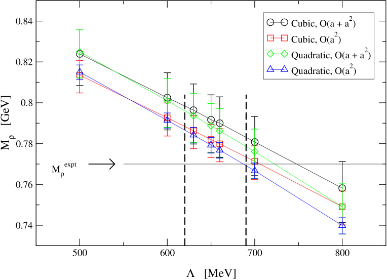
Figure 12: Variation of the physical mass of the $\rho$-meson, $M_{\rho}$, as a function of $\Lambda$, using the Adelaide approach with the scale set from $r_{0}$. The two vertical dashed lines define the range of acceptable $\Lambda$ values (620 MeV $\leq\Lambda\leq$ 690 MeV) obtained by increasing $\chi^{2}$ by unity in Fig. 11.

From a detailed examination of Table 6 and Fig. 12 we draw the following conclusions:

• The (statistical) errors in the mass estimates are typically around 1%.

• The Adelaide fitting procedure is very stable when the scale is set using $r_{0}$. When the scale is taken from the string tension, the four Adelaide fits are not in mutual agreement. The probable reason for this, as outlined in Sec. IV.3, is that using $\sigma$ to set the scale introduces significant ${\cal O}(a)$ errors.

• The Adelaide fitting procedure is quite accurate – lying at most at twice the statistical standard error from the experimental value for the $r_{0}$ case. It would require an uncertainty of only around 1-2% in $r_{0}$ (and around 2-6% in $\sqrt{\sigma}$) for the Adelaide central values to be in agreement with the experimental value of $M_{\rho}$.

• From Fig. 12, the variation of $M_{\rho}$ with $\Lambda$ is small - roughly the same order as the other uncertainties.

• The naive fitting procedure has both a larger spread of values and is further from the experimental value than the Adelaide procedure.

As a result, we conclude that the Adelaide procedure represents a significant improvement over the naive approach.

We obtain final estimates of $M_{\rho}$ by taking the the quadratic chiral extrapolation, the scale set from $r_{0}$, and ${\cal O}(a^{2})$ corrections in the $a_{0}$ coefficient in both the Adelaide and naive fitting procedure. (The reason for this choice of fit type is described in detail in Sec. IV.3.) The central value in the Adelaide case was obtained at $\Lambda=$ 655 MeV from Fig. 12 (which is an adjustment of 1 MeV from the value obtained at $\Lambda=$ 650 MeV in Table 6). The value of $\Lambda=$ 655 MeV was used since it is where the minimum of $\chi^{2}$ occurs in Fig. 11. We obtain an estimate of the error in the fit procedure from the spread in the mass predictions using $r_{0}$ for the scale (since we have reservations about the method when the string tension is used to set the scale). An estimate of the uncertainty associated with the determination of $\Lambda$ comes from varying $\chi^{2}$ by unity as described above — i.e. by reading off this error from the vertical dashed lines in Fig. 12. Finally then we are led to the following result for the physical mass of the $\rho$-meson:

$$M_{\rho}^{Adelaide} = 778(4){\scriptstyle{}^{+{16}}_{-{6}}}{\scriptstyle{}^{+{8}}_{-{9}}}\textrm{MeV,}$$ (19)

$$M_{\rho}^{Naive} = 825(4){\scriptstyle{}^{+{12}}_{-{8}}}\textrm{MeV,}$$ (20)

where the first error is statistical, the second is from the fit procedure, and, in the Adelaide case, the third error is from the determination of $\Lambda$. The second error on the Adelaide result also includes an uncertainty from the choice of finite-range regulator, which contributes $+3/-6\,{\rm MeV}$ to the error Allton:2005fb . Note that we have not included an error from the determination of $r_{0}$ itself. The only other effect which separates our analysis from nature is that the data we are analysing contains only 2 rather than 2+1 light dynamical flavours. We have no way to estimate the residual systematic error from this source once $r_{0}$ is matched to the physical value.

The fit parameters shown in Table 5 allow one to shift each of the simulation results to the infinite-volume, continuum limit and to remove the effects of partial quenching — hence restoring unitarity in the quark masses. This can be achieved by first considering the preferred form of Eq. (17), where $X_{1}=a_{6}=0$,

$$\sqrt{(M_{V}^{deg})^{2}-\Sigma_{TOT}}=(a_{0}^{cont}+X_{2}a^{2})+a_{2}(M_{PS}^{deg})^{2}+a_{4}(M_{PS}^{deg})^{4}\,.$$ (21)

This can then be used to let $M_{V}^{deg}\to M_{V}^{unit}$ at the same time as removing volume and discretisation artifacts. Rewriting Eq. (21) in terms of the fit vector meson mass gives,

$$M_{V}^{deg}(a)=\bigg{[}\left((a_{0}^{cont}+X_{2}a^{2})+a_{2}(M_{PS}^{deg})^{2}+a_{4}(M_{PS}^{deg})^{4}\right)^{2}+\Sigma_{TOT}(M_{PS}^{deg};L)\bigg{]}^{1/2}\,.$$ (22)

In the physical continuum limit, this becomes

$$M_{V}^{unit}(a\to 0)=\bigg{[}\left(a_{0}^{cont}+a_{2}(M_{PS}^{unit})^{2}+a_{4}(M_{PS}^{unit})^{4}\right)^{2}+\Sigma_{TOT}(M_{PS}^{unit};L\to\infty)\bigg{]}^{1/2}\,.$$ (23)

With the unknown parameters determined from the best fit to the entire data set, this then provides a prescription for restoring the physical limit of the data. Specifically, each of the vector meson masses (calculated at finite $a$ and $L$) are shifted by an amount

$$\delta M = \bigg{[}\left(a_{0}^{cont}+a_{2}(M_{PS}^{unit})^{2}+a_{4}(M_{PS}^{unit})^{4}\right)^{2}+\Sigma_{TOT}(M_{PS}^{unit};L\to\infty)\bigg{]}^{1/2}$$ (24)

$$-\bigg{[}\left((a_{0}^{cont}+X_{2}a^{2})+a_{2}(M_{PS}^{deg})^{2}+a_{4}(M_{PS}^{deg})^{4}\right)^{2}+\Sigma_{TOT}(M_{PS}^{deg};L)\bigg{]}^{1/2}\,.$$

Here it is understood that the pion masses that one should therefore plot against on the $x$-axis are the unitary pion, at the point where the sea mass is held fixed and the valence mass is changed, ie. $M(\beta,\kappa_{\rm sea};\kappa_{\rm val},\kappa_{\rm val})\to M(\beta,\kappa_{\rm sea};\kappa_{\rm sea},\kappa_{\rm sea})$. The final estimate of the physical point is given by

$$\left[M_{V}^{unit}(a\to 0;L\to\infty)\right]_{\rm estimate}=\left[M_{V}^{deg}\right]_{\rm lattice}+\delta M\,.$$ (25)

The results of these shifts are displayed in Fig. 13, where we observe a remarkable result. The tremendous spread of data seen in Fig. 10 is dramatically reduced, with all 80 points now lying very accurately on a universal curve.

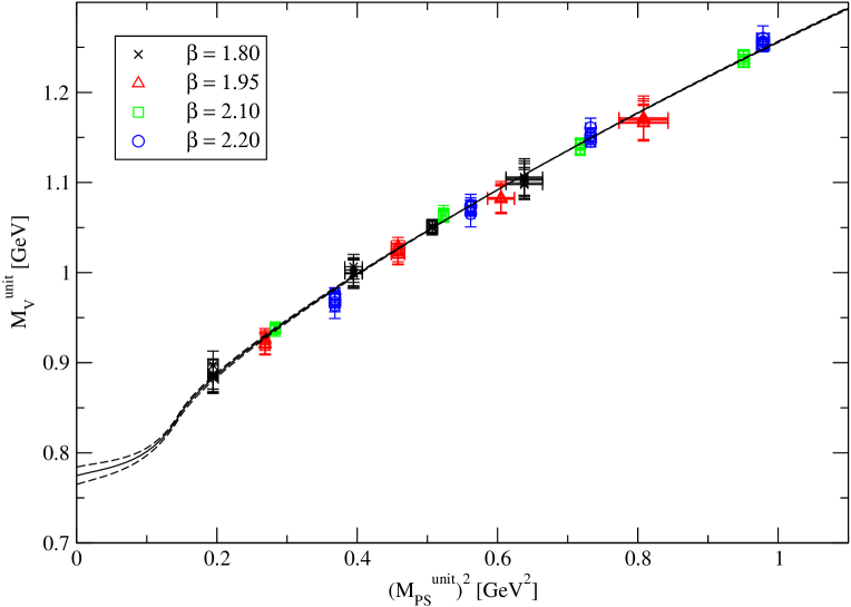
Figure 13: The same 80 lattice data points as in Fig. 10, after correction to restore the infinite-volume, continuum and quark-mass unitarity limits. The central curve displays the best-fit from the global analysis with $\Lambda=$ 655 MeV. The dashed curves show the (statistically constrained) bounds on the FRR scale, $0.620<\Lambda<0.690$ GeV.

One feature of Fig. 10 is the very steady approach to the chiral limit from the physical point. This yields a value for the vector meson mass in the chiral limit ($M_{\rho}^{0}$) that is very near the physical value. To remove the overall scale, we report on the mass shift between the physical and chiral values, finding

$$M_{\rho}-M_{\rho}^{0}=3.7(2)(4)(8)\,{\rm MeV},$$ (26)

where the sources of uncertainty are the same as those reported above for $M_{\rho}$ in Eq. (19). This small number indicates that the sigma term for the $\rho$ is significantly smaller than the nucleon, where the derivative is observed to increase near the chiral limit Leinweber:2003dg . The reduced slope in the case of the $\rho$ arises from the presence of substantial spectral strength in the low-energy two-pion channel below the $\rho$-meson mass Leinweber:1993yw .

VI Conclusions

In summary, we have tackled the ambitious task of producing a single, unified chiral fit to all of the accurate CP-PACS data for the mass of the $\rho$-meson in partially quenched QCD – i.e., the case where $\kappa_{\rm sea}\neq\kappa_{\rm val}$. As well as using a naive polynomial fit in $M_{PS}^{2}$, we have generalized the Adelaide approach, developing a unified analysis approach, to fit the data. This approach enables one to account for finite volume errors by evaluating the chiral self-energy contributions with the same momentum discretisation implicit in the lattice simulations. In addition, we have been able to quantify the residual ${\cal O}(a)$ effects and hence carry out a continuum extrapolation (c.f. Figs. 8 and 9).

The $\chi^{2}$ obtained for the Adelaide fit, with the physical scale set using $r_{0}$, is a factor of two lower than that for any other method. This provides considerable confidence in the method, even before it is used to produce the physical mass of the $\rho$. The quality of the fit leads to very small (statistical) error bars — see Table 6.

In addition, it is possible to estimate the systematic errors in the extrapolation to the physical $\rho-$mass associated with the fitting procedure (both the chiral and continuum-limit fitting procedures). In particular, the finite-range regulator parameter, $\Lambda$, is constrained by the model-independent lattice QCD data, and the variation of the $M_{\rho}$ prediction within this range was found to be 1%.

The curve through Fig. 13 displays the determined variation of the $\rho$-meson mass with pion mass. This curve also presents an extrapolation to the physical point, allowing extraction of the physical $\rho$-meson mass

$$M_{\rho}=778(4){\scriptstyle{}^{+{16}}_{-{6}}}{\scriptstyle{}^{+{8}}_{-{9}}}\,{\rm MeV},\\$$ (27)

where the first error is statistical, the second is from variations of the fit procedure and the third from the determination of $\Lambda$. Whereas the naive fitting procedure leads to a value that is 50-60 MeV too high, the result from the chiral analysis is in excellent agreement with the experimentally observed mass.

References

- (1) A. Ali Khan et al. [CP-PACS Collaboration], Phys. Rev. D 65, 054505 (2002) [Erratum-ibid. D 67, 059901 (2003)] [arXiv:hep-lat/0105015].
- (2) D. B. Leinweber, A. W. Thomas and R. D. Young, Phys. Rev. Lett. 92 (2004) 242002 [arXiv:hep-lat/0302020].
- (3) M. Procura, T. R. Hemmert and W. Weise, Phys. Rev. D 69, 034505 (2004) [arXiv:hep-lat/0309020].
- (4) D. B. Leinweber, A. W. Thomas, K. Tsushima and S. V. Wright, Phys. Rev. D 61, 074502 (2000) [arXiv:hep-lat/9906027].
- (5) S. Durr, Eur. Phys. J. C 29, 383 (2003) [arXiv:hep-lat/0208051].
- (6) C. Bernard, S. Hashimoto, D. B. Leinweber, P. Lepage, E. Pallante, S. R. Sharpe and H. Wittig, Nucl. Phys. Proc. Suppl. 119, 170 (2003) [arXiv:hep-lat/0209086].
- (7) R. D. Young, D. B. Leinweber and A. W. Thomas, Prog. Part. Nucl. Phys. 50, 399 (2003) [arXiv:hep-lat/0212031].
- (8) S. R. Beane, Nucl. Phys. B 695, 192 (2004) [arXiv:hep-lat/0403030].
- (9) A. W. Thomas, P. A. M. Guichon, D. B. Leinweber and R. D. Young, Prog. Theor. Phys. Suppl. 156, 124 (2004) [arXiv:nucl-th/0411014].
- (10) D. B. Leinweber, A. W. Thomas and R. D. Young, Nucl. Phys. A 755, 59 (2005) [arXiv:hep-lat/0501028].
- (11) J. F. Donoghue, B. R. Holstein and B. Borasoy, Phys. Rev. D 59, 036002 (1999) [arXiv:hep-ph/9804281].
- (12) D. Djukanovic, M. R. Schindler, J. Gegelia and S. Scherer, Phys. Rev. D 72, 045002 (2005).
- (13) R. D. Young, D. B. Leinweber and A. W. Thomas, Phys. Rev. D 71, 014001 (2005) [arXiv:hep-lat/0406001].
- (14) M. F. L. Golterman and K. C. L. Leung, Phys. Rev. D 57, 5703 (1998) [arXiv:hep-lat/9711033].
- (15) S. R. Sharpe and N. Shoresh, Phys. Rev. D 64, 114510 (2001) [arXiv:hep-lat/0108003].
- (16) J. W. Chen and M. J. Savage, Phys. Rev. D 65, 094001 (2002) [arXiv:hep-lat/0111050].
- (17) S. R. Beane and M. J. Savage, Nucl. Phys. A 709, 319 (2002) [arXiv:hep-lat/0203003].
- (18) D. B. Leinweber, Phys. Rev. D 69, 014005 (2004) [arXiv:hep-lat/0211017].
- (19) D. Arndt and B. C. Tiburzi, Phys. Rev. D 68, 094501 (2003) [arXiv:hep-lat/0307003].
- (20) D. Arndt and C.-J. D. Lin, Phys. Rev. D 70, 014503 (2004) [arXiv:hep-lat/0403012].
- (21) J. Bijnens, N. Danielsson and T. A. Lahde, Phys. Rev. D 70, 111503 (2004) [arXiv:hep-lat/0406017].
- (22) W. Detmold and C.-J. D. Lin, Phys. Rev. D 71, 054510 (2005) [arXiv:hep-lat/0501007].
- (23) J. Bijnens, P. Gosdzinsky and P. Talavera, Nucl. Phys. B 501, 495 (1997) [arXiv:hep-ph/9704212].
- (24) P. C. Bruns and U. G. Meissner, Eur. Phys. J. C 40, 97 (2005) [arXiv:hep-ph/0411223].
- (25) C. R. Allton, W. Armour, D. B. Leinweber, A. W. Thomas and R. D. Young, Phys. Lett. B 628, 125 (2005) [arXiv:hep-lat/0504022].
- (26) D. B. Leinweber and T. D. Cohen, Phys. Rev. D 49 (1994) 3512 [arXiv:hep-ph/9307261].
- (27) D. B. Leinweber, A. W. Thomas, K. Tsushima and S. V. Wright, Phys. Rev. D 64, 094502 (2001) [arXiv:hep-lat/0104013].
- (28) J. N. Labrenz and S. R. Sharpe, Phys. Rev. D 54, 4595 (1996) [arXiv:hep-lat/9605034].
- (29) C. K. Chow and S. J. Rey, Nucl. Phys. B 528, 303 (1998) [arXiv:hep-ph/9708432].
- (30) R. D. Young, D. B. Leinweber, A. W. Thomas and S. V. Wright, Phys. Rev. D 66, 094507 (2002) [arXiv:hep-lat/0205017].
- (31) R. Sommer, Nucl. Phys. B 411, 839 (1994) [arXiv:hep-lat/9310022]. R. G. Edwards, U. M. Heller and T. R. Klassen, Nucl. Phys. B 517, 377 (1998) [arXiv:hep-lat/9711003].
- (32) R. G. Edwards, U. M. Heller and T. R. Klassen, Phys. Rev. Lett. 80, 3448 (1998) [arXiv:hep-lat/9711052]. J. M. Zanotti, B. Lasscock, D. B. Leinweber and A. G. Williams, Phys. Rev. D 71, 034510 (2005) [arXiv:hep-lat/0405015].
- (33) O. Bär, Nucl. Phys. Proc. Suppl. 140, 106 (2005) [arXiv:hep-lat/0409123].
- (34) G. Rupak and N. Shoresh, Phys. Rev. D 66, 054503 (2002) [arXiv:hep-lat/0201019].
- (35) O. Bar, G. Rupak and N. Shoresh, Phys. Rev. D 70, 034508 (2004) [arXiv:hep-lat/0306021].
- (36) S. Aoki, Phys. Rev. D 68, 054508 (2003) [arXiv:hep-lat/0306027].
- (37) S. R. Beane and M. J. Savage, Phys. Rev. D 68, 114502 (2003) [arXiv:hep-lat/0306036].
- (38) H. R. Grigoryan and A. W. Thomas, arXiv:hep-lat/0507028.