DESY/05-206 October 2005
Two–dimensional lattice Gross–Neveu model
with Wilson twisted mass fermions

We study the two-dimensional lattice Gross–Neveu model with Wilson twisted mass fermions in order to explore the phase structure in this setup. In particular, we investigate the behaviour of the phase transitions found earlier with standard Wilson fermions as a function of the twisted mass parameter $\mu$. We find that qualitatively the dependence of the phase transitions on $\mu$ is very similar to the case of lattice QCD.

1 Introduction

Recent results from simulations of lattice QCD with Wilson twisted mass fermions [1, 2] revealed an intriguing phase structure with an Aoki phase at strong coupling [3, 4] and pronounced first order phase transitions at intermediate values of the coupling which weakens when the continuum limit is approached [5, 6, 7, 8]. These findings are supported by calculations in chiral perturbation theory for standard Wilson fermions [9] which were later extended to the case of Wilson twisted mass fermions [10, 11, 12, 13, 14, 15]. See refs. [16, 17] for reviews. The appearance of the first order phase transition turns out to be a generic phenomenon of Wilson fermions and takes place independent of whether the twisted mass parameter is switched on or not.

Of course, one may argue that on a finite lattice no phase transition can occur and that the metastabilities observed in refs. [5, 6, 7, 8] are purely an artefact of the algorithm employed. From the analytical side, chiral perturbation theory ($\chi$PT) is a powerful tool to determine the phase structure. However, the assumption of $\chi$PT is that $a\Lambda\ll 1$, where $a$ is the lattice spacing and $\Lambda$ is the scale parameter. Moreover, the analysis by $\chi$PT is done up to $O(a^{2})$ only. Thus, it is unclear whether at large values of $a$ and by inclusion of higher order terms the picture can change substantially.

Motivated by these considerations and in order to have another angle on the problem, we decided to study the phase structure of the Gross-Neveu model [18] on the lattice including a twisted mass term, taking this as a toy model of twisted mass lattice QCD. In the large-$N$ limit, where $N$ is the number of flavours, the Gross-Neveu (GN) model is asymptotically free and has bound states [18]. The GN-model is one-loop exact in the large-$N$ limit and hence, in this limit, higher order contributions of the lattice spacing are taken into account. In this sense, the large-$N$ investigation of the GN-model goes beyond $\chi$PT and can provide therefore a complementary picture of the phase diagram, although one should always keep in mind that we are considering a two-dimensional model only.

The GN-model has been studied for pure Wilson fermions in the large-$N$ limit in refs. [19, 20]. In ref. [21], the phase structure of the lattice GN-model with Wilson fermions is first predicted and a so-called Parity-Flavour broken phase (or Aoki phase) was found. A refined analysis [19] showed that even the zero temperature phase diagram is rather complex and reveals besides the second order phase transition to the Aoki phase strong first order phase transitions. In this work we want to extend the investigations of refs. [21, 20, 19] to the case when a twisted mass parameter $\mu$ is switched on. In particular, we want to address the question of the $\mu$-dependence of the first order phase transition. We hope that our findings can give some, at least qualitative insight also into the generic phase diagram of lattice QCD with Wilson fermions.

2 Lattice Gross–Neveu model with twisted mass fermion

A formulation of the two-dimensional Gross–Neveu model on the lattice with Wilson fermions is given in refs. [21, 20, 19]. Our study here follows refs. [20, 19] where the the lattice couplings of the model are treated separately. We choose the so-called twisted basis [2] for our investigation in which the Lagrangian of the model reads

$${\cal L}_{GN}=\bar{\chi}\left[\gamma\cdot\nabla^{sym}-r\nabla_{\mu}\nabla_{\mu}^{\dagger}+M_{cr}(r)+m_{q}e^{i\gamma_{5}\tau_{3}\omega}\right]\chi-\frac{g_{\sigma}^{2}}{2N}(\bar{\chi}\chi)^{2}-\frac{g_{\pi}^{2}}{2N}(\bar{\chi}i\gamma_{5}\tau_{3}\chi)^{2},$$ (1)

where $(\bar{\chi},\chi)$ denote the fermion fields in the “twisted basis” or $\chi$-basis, and $N$ is the number of the “flavours”. The parameters of the model are the critical fermion mass $M_{cr}$, the off-set fermion mass $m_{q}$, the twist angle $\omega$ and the couplings $g_{\sigma}$ and $g_{\pi}$. In this version of twisted mass fermions, the Wilson term is not twisted. An important remark is that in general the coupling constant $g_{\sigma}\neq g_{\pi}$ on the lattice[20, 19].

In momentum space, the Lagrangian in the $\chi$-basis is given as

$${\cal L}_{GN}=\bar{\chi}\left[K(p)+W(p)+m_{0}+i\gamma_{5}\tau_{3}\mu\right]\chi-\frac{g_{\sigma}^{2}}{2N}(\bar{\chi}\chi)^{2}-\frac{g_{\pi}^{2}}{2N}(\bar{\chi}i\gamma_{5}\tau_{3}\chi)^{2},$$ (2)

where $K(p)=i\sum_{\nu}\gamma_{\nu}\sin(p_{\nu}a)$, $W(p)=r\sum_{\nu}(1-\cos(p_{\nu}a))$, $m_{0}=M_{cr}+m_{q}\cos\omega$, $\mu=m_{q}\sin\omega$ and $r$ the Wilson parameter. The situation of “full twist” is realized when $\omega=\pm\pi/2$ or, equivalently, $m_{0}=M_{cr}$.

In the large-$N$ limit we obtain the Lagrangian

$${\cal L}_{GN}=\bar{\chi}\left[K(p)+W(p)+\sigma_{L}+i\gamma_{5}\tau_{3}\pi_{L}\right]\chi+\frac{N}{2g_{\sigma}^{2}}(\sigma_{L}-m_{0})^{2}+\frac{N}{2g_{\pi}^{2}}(\pi_{L}-\mu)^{2},$$ (3)

where, by the equations of motion, the bosonic fields are defined as

$$\sigma_{L}=-\frac{g_{\sigma}^{2}}{N}(\bar{\chi}\chi)+m_{0}\quad,\quad\pi_{L}=-\frac{g_{\pi}^{2}}{N}(\bar{\chi}i\gamma_{5}\tau_{3}\chi)+\mu\quad.$$ (4)

To solve the model, we integrate out the fermion fields, treating the $\pi$- and $\sigma$-fields as constant since the quantum fluctuations are suppressed in the large-$N$ limit. We then obtain the effective potential $V_{eff}$,

$$Z=\int[d\chi][d\bar{\chi}]\exp\{-\int d^{2}x{\cal L}_{GN}\}\equiv\exp\{-N\Omega V_{eff}\}\,,$$ (5)

where $\Omega$ is the space-time volume.

$V_{eff}$ in large-$N$ limit is given by (setting here and in the following $r=1$),

$$V_{eff}=\frac{1}{2g_{\sigma}^{2}}(\sigma_{L}-m_{0})^{2}+\frac{1}{2g_{\pi}^{2}}(\pi_{L}-\mu)^{2}$$ (6)

$$-\int_{p}\ln[\sum_{\nu}\sin^{2}(p_{\nu}a)+\{\sum_{\nu}(1-\cos(p_{\nu}a))\}^{2}+(\sigma_{L}^{2}+\pi_{L}^{2})+2\sigma_{L}\sum_{\nu}(1-\cos(p_{\nu}a))],$$

where $\int_{p}=\int_{-\pi}^{\pi}\frac{d^{2}(pa)}{(2\pi)^{2}}$. Note that eq. (6) has the same form as the effective potential in the Wilson fermion formulation of the GN-model on the lattice [20, 19]. The difference shows up only in the definition of the field $\pi_{L}$, where there is an explicit appearance of the twisted mass parameter $\mu$.

2.1 Phase structure and Pion mass in twisted basis

At $\mu=0$, i.e. for pure Wilson fermions, the phase structure of the Gross-Neveu model is already quite complicated showing first order and second order phase transitions. It is unclear, whether the presence of the twisted mass term can change the phase structure. In order to explore the phase structure of the lattice GN-model, it is sufficient to solve the saddle point equations as they can be derived from the effective potential $V_{eff}$.

In the following we will concentrate on the twisted basis, because then the effective potential has the same form as the one for ordinary Wilson fermion. The effect of the twisted mass parameter is, to 1-loop order, only included via the field $\pi_{L}$ by a shift.

The saddle point equations are

$$\frac{\partial V_{eff}}{\partial\sigma_{L}}=\frac{\sigma_{L}-m_{0}}{g_{\sigma}^{2}}-\sigma_{L}F(\sigma_{L},\pi_{L})-G(\sigma_{L},\pi_{L})=0,$$ (7)

$$\frac{\partial V_{eff}}{\partial\pi_{L}}=\frac{\pi_{L}-\mu}{g_{\pi}^{2}}-\pi_{L}F(\sigma_{L},\pi_{L})=0,$$ (8)

where

$$F(\sigma_{L},\pi_{L}) = \int_{p}\frac{2}{A(\sigma_{L},\pi_{L})},\quad G(\sigma_{L},\pi_{L})=\int_{p}\frac{2\sum_{\nu}(1-\cos(p_{\nu}a))}{A(\sigma_{L},\pi_{L})},$$

$$A(\sigma_{L},\pi_{L}) = (\sigma_{L}^{2}+\pi_{L}^{2})+\{\sum_{\nu}(1-\cos(p_{\nu}a))\}^{2}+\sum_{\nu}\sin^{2}(p_{\nu}a)$$

$$+2\sigma_{L}\sum_{\nu}(1-\cos(p_{\nu}a))\,.$$

In the saddle point equations the 1-loop tadpole contributions are canceled by the potential terms of $\sigma_{L}$ and $\pi_{L}$. The solution of the saddle point equations is non-trivial and will differ from the one obtained with pure Wilson fermions opening thus the possibility of new phenomena.

The neutral pion mass and the sigma particle mass are computed from the second derivative of the effective potential at the solution of the saddle point equations,

$$M_{\pi}^{2}=\frac{1}{2}\frac{\partial^{2}V_{eff}}{\partial\pi_{L}^{2}}=\frac{1}{2}\left[\frac{1}{g_{\pi}^{2}}-F(\sigma_{L},\pi_{L})-\pi_{L}\frac{\partial}{\partial\pi_{L}}F(\sigma_{L},\pi_{L})\right]\,,$$ (9)

$$M_{\sigma}^{2}=\frac{1}{2}\frac{\partial^{2}V_{eff}}{\partial\sigma_{L}^{2}}=\frac{1}{2}\left[\frac{1}{g_{\sigma}^{2}}-F(\sigma_{L},\pi_{L})-\sigma_{L}\frac{\partial}{\partial\sigma_{L}}F(\sigma_{L},\pi_{L})-\frac{\partial}{\partial\sigma_{L}}G(\sigma_{L},\pi_{L})\right].$$ (10)

Our strategy is the following. We first fix the values the couplings $g_{\sigma}^{2}$ and $g_{\pi}^{2}$ such that the perturbative tuning relation between $g_{\pi}^{2}$ and $g_{\sigma}^{2}$ as computed for the ordinary Wilson fermion formulation [19] holds,

$$\frac{1}{g_{\pi}^{2}}=\frac{1}{g_{\sigma}^{2}}+4C_{2}+O(a)\,,\quad\quad C_{2}=\frac{2\sqrt{3}}{27}+\frac{1}{12\pi}\,.$$ (11)

In the following table, the (perturbative) tuning values for various $g_{\sigma}^{2}$ are given.

$g_{\sigma}^{2}$	0.1	0.5	1.0	2.0
$g_{\pi}^{2}$	0.094	0.381	0.617	0.893

We then also fix the value of the twisted mass $\mu$ and determine the values of $\sigma_{L}$ and $\pi_{L}$ from the solutions of the saddle point equations eqs. (7, 8) as a function of $m_{0}$. In this way, we can study whether $\sigma_{L}$ or $\pi_{L}$ undergo a phase transition. Once we have the value for $\sigma_{L}$ and $\pi_{L}$ we can insert them into the gap equations, eqs. (9, 10) to compute also the corresponding masses.

Let us remark that in principle there is also an additional tuning relation between the coupling $g_{\sigma}^{2}$ and the fermion mass $m_{0}$. To explore the phase structure, we will, however, vary $m_{0}$ and hence will not make use of this tuning relation. We will also restrict ourselves to values of $g_{\sigma}^{2}\leq 2$, since for larger values of the coupling the tuning relation of eq. (11) will not hold anymore.

3 Results

In this section we will give our results obtained from the solution of the saddle point equations. We used a lattice of size $128^{2}$ and solved the equations numerically. We always checked that we indeed found the correct solutions by inspecting the extrema of the effective potential itself.

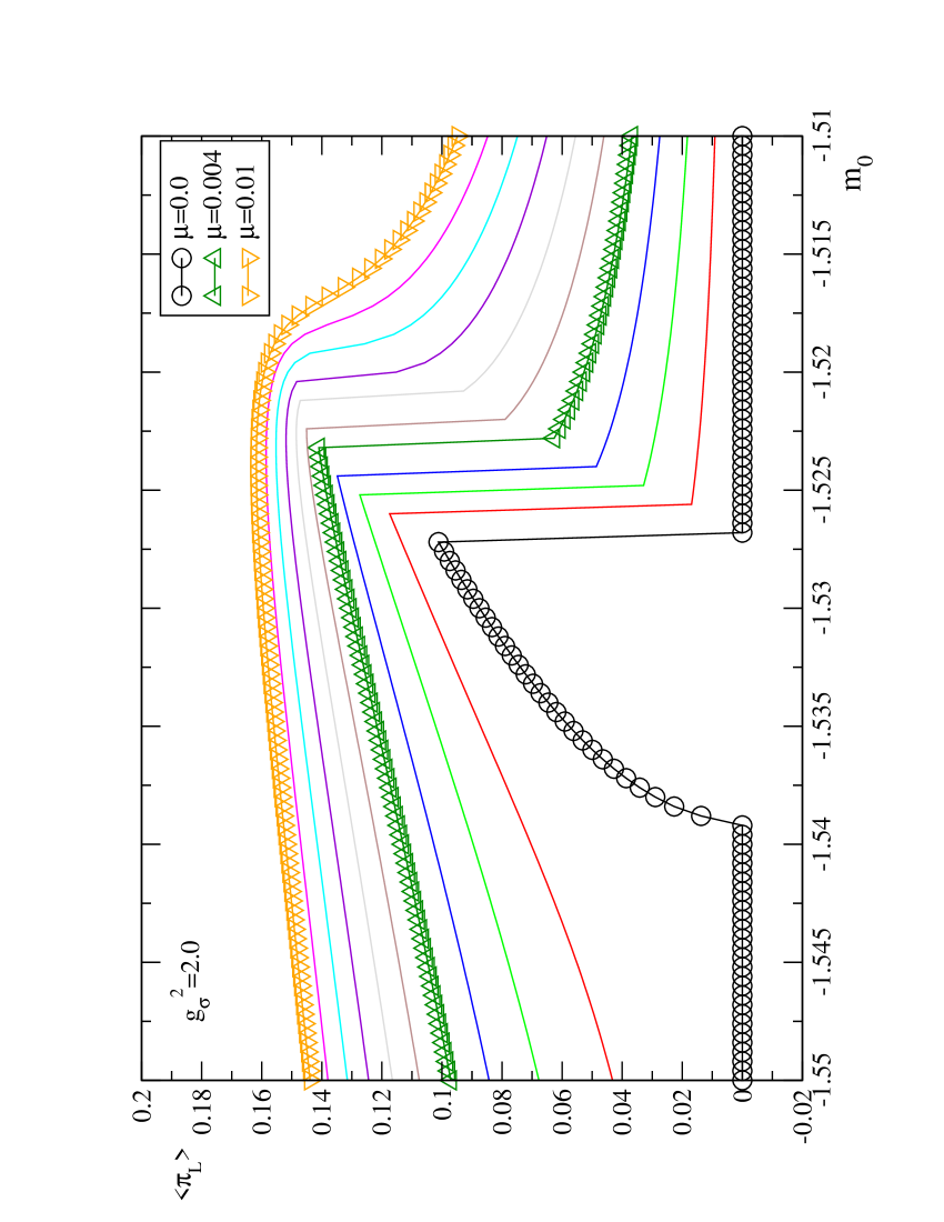
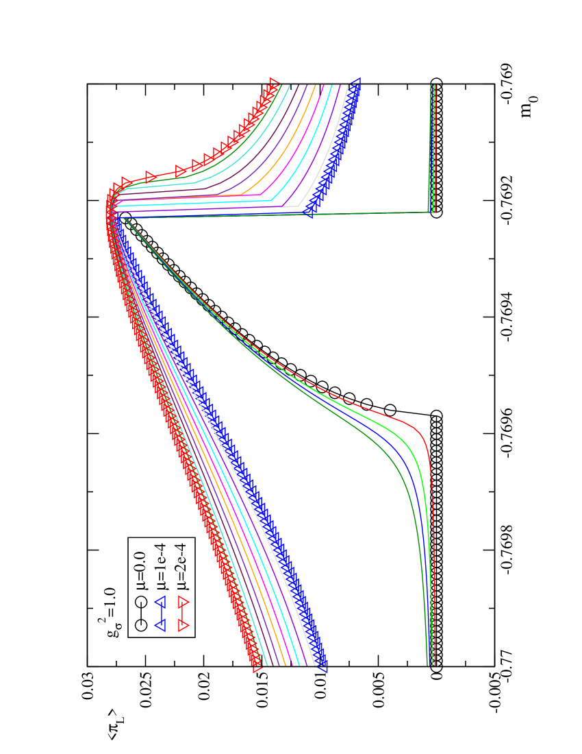
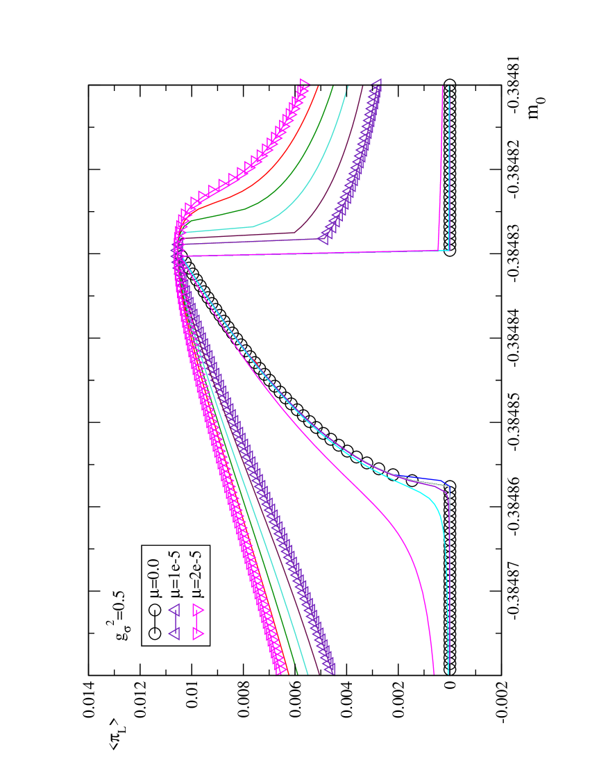
Figure 1: $\langle\pi_{L}\rangle$ as a function of the fermion mass $m_{0}$. The coupling $g_{\pi}$ is the perturbatively tuned one obtained from eq. (11) and assumes values of $g_{\pi}^{2}=0.893$, $g_{\pi}^{2}=0.617$ and $g_{\pi}^{2}=0.381$ from top to bottom. We represent some values of the twisted mass parameter $\mu$ by open symbols. Other, intermediate values of $\mu$ are represented by solid lines in the graph.

In fig. 1 we show the expectation value $\langle\pi_{L}\rangle$ of the $\pi$-field as a function of the mass parameter $m_{0}$ for various values of the twisted mass parameter $\mu$. Let us summarize the results of our large-$N$ computations. At $\mu=0$ and increasing the values of $m_{0}$, we find in accordance with ref. [19] first and second order phase transitions, where the $\pi$-field assumes a non-zero value. For larger values of $m_{0}$ there is a first order transition where $\langle\pi_{L}\rangle$ jumps back to a zero value. This structure changes in two aspects when the twisted mass parameter $\mu$ is switched on. First, the second order phase transition vanishes and $\langle\pi_{L}\rangle$ shows an analytical behaviour. Second, for some range of $\mu<\mu_{\mathrm{crit}}$ the first order phase transition remains. However, it becomes weaker when $\mu$ is increased and turns into a second order phase transition when a critical value $\mu_{\mathrm{crit}}$ is reached. For $\mu>\mu_{\mathrm{crit}}$ the phase transition disappears altogether and turns into a completely smooth and analytical behaviour.

When the coupling $g_{\sigma}^{2}$ is made smaller, with the associated tuning of $g_{\pi}^{2}$, the region in $m_{0}$ where the phase transitions occur shrinks and also the jumps at the first order phase transitions become smaller. Thus the qualitative picture does not change when we approach the continuum limit. Note that also the value of $\mu_{\mathrm{crit}}$ gets smaller with decreasing coupling $g_{\sigma}^{2}$.

The fate of the first order phase transition is very much reminiscent of the situation of four-dimensional lattice QCD. Also there it has been found from numerical simulations [7, 6, 5] and from calculations in chiral perturbation theory [9, 12, 10, 11, 15] that the first order phase transition terminates at a critical values of $\mu$. Note that the values of $m_{0}$ where the first order phase transition takes place moves to larger values when $\mu$ is increased. A similar phenomenon can be expected also in lattice QCD. What is very interesting from our analysis in the GN-model –and apparently different from current findings of lattice QCD and $O(a^{2})$-$\chi$PT– is that this first order phase transition is accompanied by a second order phase transition at $\mu=0$ or its remnant at $\mu>0$.

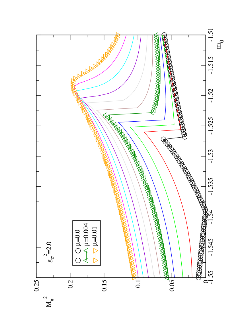
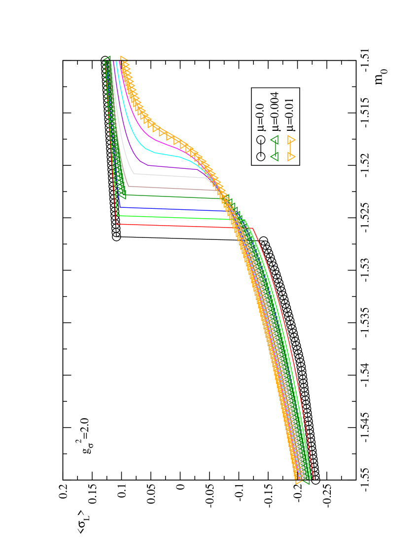
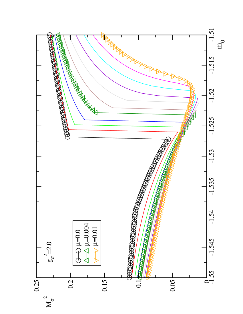
Figure 2: We show (from top to bottom) the pion mass, the $\sigma$-field expectation value and the $\sigma$-mass as a function of $m_{0}$ at $g_{\sigma}^{2}=2$, $g_{\pi}^{2}=0.893$.

In fig. 2 we show at the example of the coupling values $g_{\sigma}^{2}=2$, $g_{\pi}^{2}=0.893$ the behaviour of the pion mass (top), the $\sigma$-field expectation value (middle) and the $\sigma$-mass (bottom). At $\mu=0$ and increasing $m_{0}$, the pion mass first goes to zero and vanishes at the second order phase transition. It then assumes non-zero values again until it jumps when the first order phase transition is hit. Switching on $\mu$, the second order phase transition vanishes and the behaviour of the pion mass becomes continuous. The first order phase transition remains, however, until $\mu=\mu_{\mathrm{crit}}$. For larger values of $\mu$ also the first order phase transition vanishes and the pion mass shows an overall analytical behaviour.

The $\sigma$-field expectation value and mass do not show a large sensitivity on the second order phase transition. However, this field feels the first order phase transition strongly and shows jumps in the field expectation value as well as in the mass. The picture shown here for the couplings $g_{\sigma}^{2}=2$, $g_{\pi}^{2}=0.893$ stays qualitatively unchanged when the coupling $g_{\sigma}^{2}$ is reduced with the associated tuning of $g_{\pi}^{2}$.

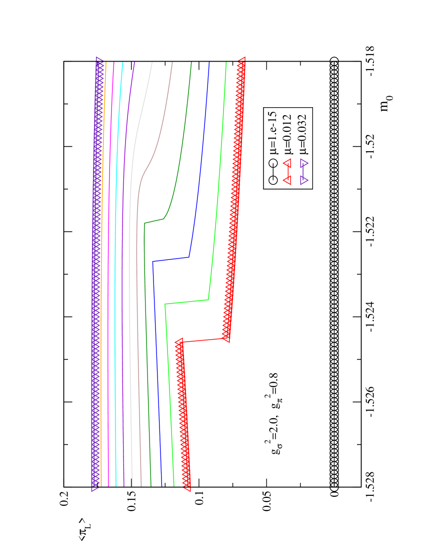
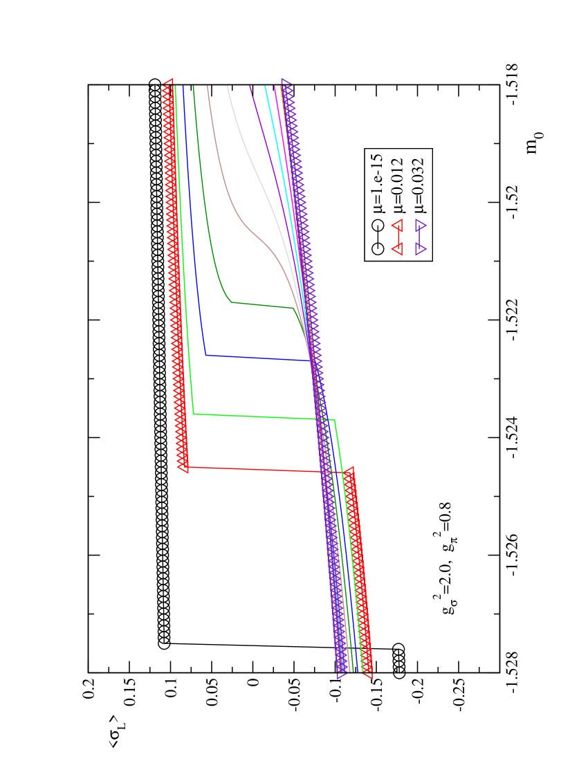
Figure 3: The $\pi$- (top) and $\sigma$-field (bottom) expectation values as a function of $m_{0}$ at the so-called $\sigma$-phase transition [19].

Finally and for completeness, we show in fig. 3 the fate of the so-called $\sigma$-phase transition [19] for a value of the coupling $g_{\sigma}^{2}=2$. Note that the value of the coupling is now $g_{\pi}^{2}=0.8$ and does not correspond to the ones of the perturbative tuning. This phase transition is characterized by the fact that at $\mu=0$ the $\sigma$-field expectation value $\langle\sigma_{L}\rangle$ shows a discontinuous jump, whereas the $\pi$-field expectation value stays essentially zero. This phase transition survives when $\mu$ is switched on and can clearly be seen in the jump of $\langle\sigma_{L}\rangle$. It is interesting to observe that the point in $m_{0}$ where this jumps happens is moved to larger values of $m_{0}$ when $\mu$ is increased. However, also for this case the phase transition vanishes when $\mu$ is increased above a certain critical value. Furthermore, the $\pi$-field shows now at $\mu>0$ also a jump and exhibits the first order phase transition.

4 Summary

Following the earlier work of refs. [21, 20, 19] we studied in this letter, how the presence of the twisted mass term influences the known phase diagram of the two-dimensional Gross–Neveu model which we consider as a toy model of lattice QCD. We found that the coexistence of the Aoki phase and the first order phase transition as it is obtained at vanishing twisted mass parameter $\mu$ [19] is not kept at $\mu>0$. The first change is that at $\mu>0$ the second order phase transition turns into a smooth and analytical behaviour, although e.g. the $\pi$-field expectation $\langle\pi_{L}\rangle$ still shows a rapid change. The second change is that the gap in $\langle\pi_{L}\rangle$ of the first order phase transition shrinks with increasing values of $\mu$ and finally vanishes at a critical value of $\mu=\mu_{\mathrm{crit}}$. In addition, the values of $m_{0}$, where the first order phase transition takes place, is shifted to larger values when $\mu$ is increased.

The motivation of our investigation has been to provide a complementary analysis of a “QCD-like” model to the findings of numerical simulations [5, 6, 7, 8] and from (Wilson) chiral perturbation theory [9, 10, 11, 12, 13, 14, 15]. Both of these approaches have some shortcomings: in the numerical simulations it is not clear whether the metastability effects are due to a bad behaviour of the algorithms employed. $\chi$PT on the other hand can, in principle, only predict the phase structure reliably in a region close to the continuum limit where the $O(a^{2})$ expansion is valid and the quark masses are small.

Our findings from the large-$N$ analysis of the GN-model as described above show a striking similarity to the results from the four-dimensional simulations and from $\chi$PT. This includes the shift in the critical mass, the weakening of the first order phase transition as function of increasing $\mu$ and the vanishing of the first order phase transition altogether when $\mu>\mu_{\mathrm{crit}}$. However, there is also a very noticeable and important difference to the picture we have presently in four-dimensions: this concerns the coexistence of the first order phase transition with a second order transition to the Aoki phase. It is unclear to us whether this difference is an artefact of the GN-model in the large-$N$ analysis. Another, very interesting possibility is of course that so far both, the numerical simulations and the analysis in $\chi$PT have missed this possibility. Clearly, if the Aoki phase transition is very close to the first order phase transition it will be very difficult for the numerical simulations to resolve both. It could be speculated that the coexistence of both phases will show up in $\chi$PT only when higher orders are taken into account. From our analysis here we would just like to give a warning that maybe the phase structure of Wilson lattice QCD is even more complicated than our present picture suggests. If the picture of the phase diagram from our analysis in the GN-model would be correct also for lattice QCD, it would provide an argument for using a non-vanishing twisted mass parameter, since then one would avoid the complication of the existence of two phase transitions.

We also want to mention that the $\sigma$-phase transition, which is present in the GN-model with Wilson fermion, changes to a normal first order phase transition, when $\mu$ is switched on.

In this letter we did not address a number of additional interesting points that would deserve a further investigation: in order to determine the phase transition, in particular in order to study the second order phase transition, the second moment, for instance the susceptibility, may be better. In principle one could also study the scaling behaviour of physical quantities analytically toward the continuum limit. In addition, an analysis within perturbation theory could provide important insight into the renormalization properties of the GN-model with the twisted mass term.

Finally, it would be straightforward to change the discretization of the fermions in the GN-model. For example, one could study a chiral invariant GN-model. In this way, it would be possible to learn how the change of the fermion part of the action changes the phase structure. This is clearly important for four-dimensional lattice QCD simulations.

References

- [1] ALPHA, R. Frezzotti, P. A. Grassi, S. Sint and P. Weisz, JHEP 08, 058 (2001), [hep-lat/0101001].
- [2] R. Frezzotti and G. C. Rossi, JHEP 08, 007 (2004), [hep-lat/0306014].
- [3] E.-M. Ilgenfritz, W. Kerler, M. Muller-Preussker, A. Sternbeck and H. Stuben, Phys. Rev. D69, 074511 (2004), [hep-lat/0309057].
- [4] A. Sternbeck, E.-M. Ilgenfritz, W. Kerler, M. Muller-Preussker and H. Stuben, Nucl. Phys. Proc. Suppl. 129, 898 (2004), [hep-lat/0309059].
- [5] F. Farchioni et al., Eur. Phys. J. C39, 421 (2005), [hep-lat/0406039].
- [6] F. Farchioni et al., Nucl. Phys. Proc. Suppl. 140, 240 (2005), [hep-lat/0409098].
- [7] F. Farchioni et al., hep-lat/0410031.
- [8] F. Farchioni et al., hep-lat/0506025.
- [9] S. R. Sharpe and J. Singleton, Robert, Phys. Rev. D58, 074501 (1998), [hep-lat/9804028].
- [10] G. Münster, JHEP 09, 035 (2004), [hep-lat/0407006].
- [11] L. Scorzato, Eur. Phys. J. C37, 445 (2004), [hep-lat/0407023].
- [12] S. R. Sharpe and J. M. S. Wu, Phys. Rev. D71, 074501 (2005), [hep-lat/0411021].
- [13] S. R. Sharpe and J. M. S. Wu, Phys. Rev. D70, 094029 (2004), [hep-lat/0407025].
- [14] S. Aoki and O. Bär, Phys. Rev. D70, 116011 (2004), [hep-lat/0409006].
- [15] S. R. Sharpe, hep-lat/0509009.
- [16] R. Frezzotti, Nucl. Phys. Proc. Suppl. 140, 134 (2005), [hep-lat/0409138].
- [17] A. Shindler, Talk presented at Lattice 2005, Dublin, Ireland .
- [18] D. J. Gross and A. Neveu, Phys. Rev. D10, 3235 (1974).
- [19] T. Izubuchi, J. Noaki and A. Ukawa, Phys. Rev. D58, 114507 (1998), [hep-lat/9805019].
- [20] S. Aoki and K. Higashijima, Prog. Theor. Phys. 76, 521 (1986).
- [21] S. Aoki, Phys. Rev. D30, 2653 (1984).
- [22] S. Aoki, Private communication .