Glueball Spectrum and Matrix Elements on Anisotropic Lattices

Abstract

The glueball-to-vacuum matrix elements of local gluonic operators in scalar, tensor, and pseudoscalar channels are investigated numerically on several anisotropic lattices with the spatial lattice spacing ranging from 0.1fm - 0.2fm. These matrix elements are needed to predict the glueball branching ratios in $J/\psi$ radiative decays which will help identify the glueball states in experiments. Two types of improved local gluonic operators are constructed for a self-consistent check and the finite volume effects are studied. We find that lattice spacing dependence of our results is very weak and the continuum limits are reliably extrapolated, as a result of improvement of the lattice gauge action and local operators. We also give updated glueball masses with various quantum numbers.

I Introduction

Glueballs, predicted by QCD, are so exotic from the point of view of naive quark model that their existence will be a direct support of QCD. However, experimental efforts in searching for glueballs are confronted with the difficulty of identifying glueballs unambiguously, even though there are several candidate glueball resonances, such as $f_{0}(1370)$, $f_{0}(1500)$, $f_{0}(1710)$, and $f_{J}(2220)$, etc.. The key problem is that there is little knowledge of the nature of glueballs and confined QCD vacuum, which requires reliable nonperturbative methods to be implemented. The numerical study of lattice QCD, which starts from the first principles, has been playing an important role in this hot field in the last twenty years, and extensive numerical studies have been carried out to calculate the glueball spectrum berg ; old1 ; old2 ; old3 . These studies give the result that the masses of the lowest-lying glueballs range from $1\,{\rm GeV}$ to $3\,{\rm GeV}$, and suggest that the $J/\psi$ radiative decays be an ideal hunting ground for glueballs. However, apart from the mass spectrum, more characteristics are desired in order to determine glueballs in the final states of $J/\psi$ radiative decays, one of which is the partial widths of $J/\psi$ decaying into glueballs. The first step to estimate these partial widths is to calculate the vacuum-to-glueball transition matrix elements(TME) of local gluonic operators, which are nonperturbative quantities and can be investigated by the numerical calculation of lattice gauge theory.

The techniques of lattice calculations in the glueball sector have been substantially improved in the past decade. It is known that very large statistics are necessary in order for the correlation functions of gluonic operators to be measured precisely by Monte-Carlo simulation. This prohibits the lattice size being too large. On the other hand, because of the large masses of glueballs, the lattice spacing (at least in the temporal direction) has to be small enough so that reliable signals can be measured before they are undermined by statistical fluctuations. This dilemma is circumvented by using anisotropic lattices, which are spatially coarse and temporally fine. The potentially large lattice artifacts owing to the spatially coarse lattice can be suppressed by the implementation of improved lattice gauge actions. These techniques has been verified to be efficient in the calculations of glueball spectrum old3 , and are adopted as the basic formalism of this work.

The glueball matrix elements computed in this work are of the form $\langle 0|g^{2}{\rm Tr}G_{\mu\nu}G_{\rho\sigma}(x)|G\rangle$, where $|G\rangle$ refers to the glueball state with specific quantum number $J^{PC}=0^{++}$, $2^{++}$, or $0^{-+}$, $G_{\mu\nu}(x)$ is the gauge field strength, and $g$ the gauge coupling. The lattice version of the gluonic operators $g^{2}{\rm Tr}G_{\mu\nu}G_{\rho\sigma}(x)$ are constructed by the smallest Wilson loops on the lattice. To reduce lattice artifacts, the lattice version of each local gluonic operator is improved by eliminating the $O(a_{s}^{2})$ ($a_{s}$ here is the spatial lattice spacing), while the glueball states $|G\rangle$ are obtained by smeared gluonic operators. In order to get a reliable continuum extrapolation, five independent calculations are carried out on lattices with spatial lattice spacings ranging from 0.09 fm to 0.22 fm. As by-products, we also calculate the masses of the lowest-lying stationary states in all of the symmetry channels allowed on a cubic lattice at each lattice spacing. To study the systematic error from finite volume, two extra independent studies are performed at $\beta=2.4$ with the same input parameters but different lattice size. Note that the local operators mentioned above are all bare operators, they need to be renormalized to give the physical matrix elements. In this work, the renormalization constants of the scalar and tensor gluonic operators at the largest lattice spacing are extracted by the calculations of gluonic three-point functions on a much larger statistical sample (100,000 measurements). The pseudoscalar operator renormalization is determined through the calculation of the topological susceptibility. Finally, we give the nonperturbatively calculated and phenomenologically significant matrix elements.

This paper is organized as follows. In Section II, we give a detailed description of the construction of lattice local gluonic operators. Two types of lattice realization in each channel are defined, including the improvement schemes. The details of the computation, including the generation of the gauge configurations, the construction of the smeared glueball correlators, the extraction of glueball masses from the correlation functions, and the determination of the lattice spacing, are described in Sec. III. In Sec. IV, we estimate the finite volume errors and some other systematical errors. The removal of lattice artifacts due to the finite lattice spacing, including the extrapolations to the continuum limit, is described in Sec. V. The calculation of three point function and the calculation of renormalization constants are described in Sec. VI. Sec. VII gives the conclusion and some discussion.

II Local Gluonic Operators and Matrix Elements

In the continuum theory, the lowest-dimensional gauge invariant gluonic operators are of the form $g^{2}TrG_{\mu\nu}G_{\rho\sigma}$, of which the most commonly studied ones are the scalar $S(x)$ (QCD trace anomaly), the pseudoscalar $P(x)$ (topological charge density), and the tensor $\Theta_{\mu\nu}(x)$ (energy-momentum density). They all have dimension four and are all positive under charge conjugation. The explicit forms of them are

$$S(x) = g^{2}{\rm Tr}G_{\mu\nu}(x)G_{\mu\nu}(x),$$

$$P(x) = g^{2}\epsilon_{\mu\nu\rho\sigma}{\rm Tr}G_{\mu\nu}(x)G_{\rho\sigma}(x),$$

$$\Theta_{\mu\nu}(x) = 2g^{2}{\rm Tr}(G_{\mu\alpha}(x)G_{\alpha\nu}(x)-\frac{1}{4}\delta_{\mu\nu}G^{2}(x)).$$ (1)

If we introduce the chromo-electric and chromo-magnetic fields,

$$E_{i}=G_{i0}~{}~{}~{}{\rm and}~{}~{}~{}B_{i}=-\frac{1}{2}\epsilon_{ijk}G_{jk},$$ (2)

the Lorentz scalar $S(x)$ and pseudoscalar $P(x)$ can be expressed explicitly by these operators,

$$S(x) = 2g^{2}{\rm Tr}({\bf B}(x)^{2}+{\bf E}(x)^{2}),$$

$$P(x) = 8g^{2}{\rm Tr}({\bf E}(x)\cdot{\bf B}(x)),$$

$$\Theta_{ij}(x) = 2g^{2}{\rm Tr}(\theta_{ij}^{B}(x)-\theta_{ij}^{E}(x)),$$ (3)

where $\theta^{E}$ and $\theta^{B}$ are the traceless, symmetric chromo-electric and magnetic tensors,

$$\theta_{ij}^{E} = {\rm Tr}E_{i}E_{j}-\frac{1}{3}\delta_{ij}{\rm Tr}{\bf E}^{2}$$

$$\theta_{ij}^{B} = {\rm Tr}B_{i}B_{j}-\frac{1}{3}\delta_{ij}{\rm Tr}{\bf B}^{2}.$$ (4)

The scalar operators ${\rm Tr}{\bf B}^{2}(x)$ and ${\rm Tr}{\bf E}^{2}(x)$, the pseudoscalar ${\rm Tr}{\bf E}(x)\cdot{\bf B}(x)$, and the tensors $\theta^{E}$, $\theta^{B}$, are all irreducible representations of the three-dimensional rotation group $SO(3)$.

Denoting the normalized scalar, pseudoscalar, and the tensor glueball states as $|S\rangle$, $|P\rangle$, and $|T_{ij}\rangle$, respectively, the non-zero glueball-to-vacuum matrix elements for their annihilation at rest by these operators are

$$(2\pi)^{3}\delta^{3}({\bf 0})f_{(S,B)} = g^{2}\langle 0|\int d^{3}x{\rm Tr}{\bf B}^{2}(x)|S\rangle$$

$$(2\pi)^{3}\delta^{3}({\bf 0})f_{(S,E)} = g^{2}\langle 0|\int d^{3}x{\rm Tr}{\bf E}^{2}(x)|S\rangle$$

$$(2\pi)^{3}\delta^{3}({\bf 0})f_{(T,B)} = g^{2}\langle 0|\int d^{3}x{\rm Tr}\theta_{ij}^{B}(x)|T_{ij}\rangle$$

$$(2\pi)^{3}\delta^{3}({\bf 0})f_{(T,E)} = g^{2}\langle 0|\int d^{3}x{\rm Tr}\theta_{ij}^{E}(x)|T_{ij}\rangle$$

$$(2\pi)^{3}\delta^{3}({\bf 0})f_{(PS)} = g^{2}\langle 0|\int d^{3}x{\rm Tr}{\bf E}(x)\cdot{\bf B}(x)|P\rangle,$$ (5)

where no implicit summation is applied. It is straightforward to reproduce the matrix elements of the scalar $S(x)$ and pseudoscalar operator $P(x)$ by these quantities, but for the Lorentz tensor $\Theta_{\mu\nu}$, the situation is more complicated. First of all, any hadron state $|h\rangle$ is an eigenstate of $\Theta_{0\mu}$, so that the matrix elements $\langle 0|\Theta_{0\mu}(x)|h\rangle$ are zero. Together with the traceless property ($\sum\limits_{\mu}\Theta_{\mu\mu}=0$), the above condition implies that $\langle 0|\sum\limits_{i}\Theta_{ii}(x)|h\rangle$ is zero. Therefore, there are only five linearly independent no-zero matrix elements of $\Theta_{\mu\nu}$, which can be decomposed into the color-magnetic part and the color-electric part,

$$\langle 0|\Theta_{ij}(x)|T_{ij}\rangle=2\langle 0|\theta_{ij}^{B}(x)-\theta_{ij}^{E}(x)|T_{ij}\rangle.$$ (6)

Due to the rotational invariance, the five polarizations give the same matrix element of the tensor.

The Lorentz invariance is broken on the spacetime lattice. The zero-momentum stationary glueball state on the lattice must be an irreducible representation (irrep) of the lattice symmetry group, i.e. the 24-element octahedral point group $O$. The irreps of group $O$ are classified as $A_{1}$, $A_{2}$, $E$, $T_{1}$ and $T_{2}$, which are the counterparts of angular momentum $J$ for the $SO(3)$ rotational group and have dimensions 1, 1, 2, 3, and 3, respectively. Together with parity $P$ and charge conjugate $C$ transformations, the full symmetry group of simple cubic lattice is $O\bigotimes P\bigotimes C$ and the total quantum number of the lattice glueball state is $R^{PC}$, where $R$ stands for $A_{1},A_{2},E,T_{1}$ or $T_{2}$, and $PC$ can be $++$,$+-$,$-+$, or $--$. As mentioned above, we are interested in the matrix elements of the scalar, pseudoscalar, and tensor operators, which correspond to the irreps $R^{PC}$ through the following relation: $0^{++}\leftrightarrow A_{1}^{++}$, $0^{-+}\leftrightarrow A_{1}^{-+}$, and $2^{++}\leftrightarrow E^{++}\oplus T_{2}^{++}$. The zero-momentum operators are obtained by summing up all the local operators on the same time-slice in each channel. The dimensionless lattice operators are given below explicitly.

The magnetic and electric scalar (labeled $(S,B)$ and $(S,E)$ respectively) belong to the $A_{1}^{++}$ representation and are defined as

$$O^{(S,B)}(t) = \frac{g^{2}a_{s}^{4}}{L^{3}}\sum_{{\bf x}_{i}}{\rm Tr}{\bf B}^{2}({\bf x}_{i},t),$$

$$O^{(S,E)}(t) = \frac{g^{2}a_{s}^{4}}{L^{3}}\sum_{{\bf x}_{i}}{\rm Tr}{\bf E}^{2}({\bf x}_{i},t),$$ (7)

while the pseudoscalar (labeled $(P)$) belongs to the $A_{1}^{-+}$ representation and is defined as

$$O^{(PS)}(t)=\frac{g^{2}a_{s}^{4}}{L^{3}}\sum_{{\bf x}_{i}}{\rm Tr}{\bf E}({\bf x}_{i},t)\cdot{\bf B}({\bf x}_{i},t).$$ (8)

In the above questions, $L^{3}$ is the dimensionless spatial volume of the lattice and $a_{s}$ the spatial lattice spacing. For the spin-two irrep of $SO(3)$, the five polarizations are split across the $E$ and $T_{2}$ irreps of $O$ and so the tensor operators must be decomposed into their $E$ and $T_{2}$ irreducible contents. The four resulting lattice operators are labeled $(E,B)$, $(E,E)$, $({T_{2}},B)$, and $({T_{2}},E)$, and are given in terms of their continuum counterparts as

$$O_{1}^{({T_{2}},B)}(t) = \frac{g^{2}a_{s}^{4}}{L^{3}}\sum_{{\bf x}_{i}}{\rm Tr}B_{2}B_{3}({\bf x}_{i},t)$$

$$O_{2}^{({T_{2}},B)}(t) = \frac{g^{2}a_{s}^{4}}{L^{3}}\sum_{{\bf x}_{i}}{\rm Tr}B_{3}B_{1}({\bf x}_{i},t)$$

$$O_{3}^{({T_{2}},B)}(t) = \frac{g^{2}a_{s}^{4}}{L^{3}}\sum_{{\bf x}_{i}}{\rm Tr}B_{1}B_{2}({\bf x}_{i},t)$$

$$O_{1}^{({T_{2}},E)}(t) = \frac{g^{2}a_{s}^{4}}{L^{3}}\sum_{{\bf x}_{i}}{\rm Tr}E_{2}E_{3}({\bf x}_{i},t)$$

$$O_{2}^{({T_{2}},E)}(t) = \frac{g^{2}a_{s}^{4}}{L^{3}}\sum_{{\bf x}_{i}}{\rm Tr}E_{3}E_{1}({\bf x}_{i},t)$$

$$O_{3}^{({T_{2}},E)}(t) = \frac{g^{2}a_{s}^{4}}{L^{3}}\sum_{{\bf x}_{i}}{\rm Tr}E_{1}E_{2}({\bf x}_{i},t)$$ (9)

$$O_{1}^{(E,B)}(t) = \frac{g^{2}a_{s}^{4}}{L^{3}}\sum_{{\bf x}_{i}}\frac{1}{2}{\rm Tr}[B_{1}^{2}-B_{2}^{2}]({\bf x}_{i},t)$$

$$O_{2}^{(E,B)}(t) = \frac{g^{2}a_{s}^{4}}{L^{3}}\sum_{{\bf x}_{i}}\frac{1}{2\sqrt{3}}{\rm Tr}[2B_{3}^{2}-B_{1}^{2}-B_{2}^{2}]({\bf x}_{i},t)$$

$$O_{1}^{(E,E)}(t) = \frac{g^{2}a_{s}^{4}}{L^{3}}\sum_{{\bf x}_{i}}\frac{1}{2}{\rm Tr}[E_{1}^{2}-E_{2}^{2}]({\bf x}_{i},t)$$

$$O_{2}^{(E,E)}(t) = \frac{g^{2}a_{s}^{4}}{L^{3}}\sum_{{\bf x}_{i}}\frac{1}{2\sqrt{3}}{\rm Tr}[2E_{3}^{2}-E_{1}^{2}-E_{2}^{2}]({\bf x}_{i},t)$$

where the coefficients guarantee that the five components are normalized. Thus we have seven different matrix elements to be calculated on the lattice,

$$T(S,B) = \langle 0|O^{(S,B)}|A_{1}^{++}\rangle$$

$$T(S,E) = \langle 0|O^{(S,E)}|A_{1}^{++}\rangle$$

$$T(E,B) = \frac{1}{2}\langle 0|O_{1}^{(E,B)}+O_{2}^{(E,B)}|E^{++}\rangle$$

$$T(E,E) = \frac{1}{2}\langle 0|O_{1}^{(E,E)}+O_{2}^{(E,E)}|E^{++}\rangle$$

$$T(T_{2},B) = \frac{1}{3}\langle 0|O_{1}^{(T_{2},B)}+O_{2}^{(T_{2},B)}+O_{3}^{(T_{2},B)}|T_{2}^{++}\rangle$$

$$T(T_{2},E) = \frac{1}{3}\langle 0|O_{1}^{(T_{2},E)}+O_{2}^{(T_{2},E)}+O_{3}^{(T_{2},E)}|T_{2}^{++}\rangle$$

$$T(PS) = \langle 0|O^{(PS)}|A_{1}^{-+}\rangle$$ (11)

However, in the practical lattice study, the operators $O^{R}(t)$ ( with $R$ representing the labels mentioned above) are not constructed directly by $B_{i}$ or $E_{i}$, but by the proper combinations of different Wilson loops. The first definition is based on the linearly combination of a set of basic Wilson loops with the requirement that the small-$a$ expansion of each combination give the correct continuum form shown respectively in Eq. (II)-(II). We call the local operators through this definition Type-I operators. The second construction is that the lattice version of $B_{i}$ and $E_{i}$ are defined first by Wilson loops and are used to compose the local operators according to Eq. (II)-(II). The local operators through this construction is denoted Type-II.

The following details the constructions of Type-I and Type-II local operators on the anisotropic lattice with the spatial lattice spacing $a_{s}$ and the temporal lattice spacing $a_{t}$. With the tadpole improvement lepage , the tree-level Symanzik’s improvement scheme is implemented to reduce the lattice artifact in defining the local operators. Since the aspect ratio of the anisotropic lattice, $\xi=a_{s}/a_{t}$, is always set to be much larger than 1, the leading discretization errors in the local operators are at $O(a_{t}^{2},a_{s}^{4},\alpha_{s}a_{s}^{2})$ in this work.

A. Type-I Operator

Figure 1: Wilson loops used in making the Type-I gluonic operators.

Table 1: The Wilson loops used in the construction of the Type-I gluonic operators. They are illustrated by the ordered paths in the table, where $X$,$Y$,$Z$, and $T$ are directions and the minus sign indicates the path going in the negative direction of that axis. ($l_{s}$,$l_{t}$) give the numbers of the spatial and temporal links involved in the Wilson loop. These numbers also give the powers of the tadpole parameter.

Index	Name	Prototype path	No. of Links
i		$C_{i,1}$	($l_{s}$,$l_{t}$)
1	S-Plaquette	[X,Y,-X,-Y]	(4,0)
2	S-Rectangle	[X,X,Y,-X,-X,-Y]	(6,0)
3	T-Plaquette	[X,T,-X,-T]	(2,2)
4	T-Rectangle	[X,X,T,-X,-X,-T]	(4,2)
5	S-Chair	[X,Y,-X,Z,-Y,-Z]	(6,0)
6	S-Butterfly	[X,Y,-X,-Y,Z,-Y,-Z,Y]	(8,0)
7	S-Sunbed	[X,X,Y,-X,-X,Z,-Y,-Z]	(8,0)
8	T-Chair	[X,T,-X,Z,-T,-Z]	(4,2)
9	T-Sunbed	[X,X,T,-X,-X,Z,-T,-Z]	(6,2)
10	Knot	[X,T,-X,-T,Z,-Y,-Z,Y]	(6,2)
11	LS-Knot	[X,T,-X,-T,Z,Z,-Y,-Z,-Z,Y]	(8,2)
12	LT-Knot	[X,X,T,-X,-X,-T,Z,-Y,-Z,Y]	(8,2)

The Type-I operators are constructed from a set of basic Wilson loops as illustrated in Fig. 1 and Table 1, which are chosen by the requirement that the first terms of the small-$a$ expansion of these loops give the desired continuum operator forms discussed above. We take following steps in the construction. First, this set of Wilson loops are acted on by the 24 symmetry operations of the cubic point group $O$ (as listed in the Table 2), resulting in 24 copies with different orientations for each type of Wilson loops. Next, they are linearly combined to realize the irreps of the group $O$. The coefficients for each irreps, say, $A_{1}$, $E$, and $T_{2}$, are listed in Table 3. To reduce the lattice artifact due to the finite lattice spacing, the tree level Symanzik’s improvement is used, which means that differently shaped Wilson loops are combined to construct one operator so that the lattice artifacts are pushed to higher order of lattice spacing. Tadpole improvement is also implemented to improve the reliability of the lattice spacing expansion at the tree level lepage .

Table 2: The 24 symmetric operations of the cubic point group $O$ are represented by the coordinate transformation.

Index	Operation	Index	Operation
1	$(x,y,z)\rightarrow(x,y,z)$	13	$(x,y,z)\rightarrow(-z,y,x)$
2	$(x,y,z)\rightarrow(-z,-y,-x)$	14	$(x,y,z)\rightarrow(-x,-y,z)$
3	$(x,y,z)\rightarrow(z,x,y)$	15	$(x,y,z)\rightarrow(-y,x,z)$
4	$(x,y,z)\rightarrow(-y,-x,-z)$	16	$(x,y,z)\rightarrow(-z,-x,y)$
5	$(x,y,z)\rightarrow(y,z,x)$	17	$(x,y,z)\rightarrow(-x,z,y)$
6	$(x,y,z)\rightarrow(-x,-z,-y)$	18	$(x,y,z)\rightarrow(-y,-z,x)$
7	$(x,y,z)\rightarrow(z,y,-x)$	19	$(x,y,z)\rightarrow(-x,y,-z)$
8	$(x,y,z)\rightarrow(x,-y,-z)$	20	$(x,y,z)\rightarrow(z,-y,x)$
9	$(x,y,z)\rightarrow(y,x,-z)$	21	$(x,y,z)\rightarrow(-z,x,-y)$
10	$(x,y,z)\rightarrow(z,-x,-y)$	22	$(x,y,z)\rightarrow(y,-x,z)$
11	$(x,y,z)\rightarrow(x,z,-y)$	23	$(x,y,z)\rightarrow(-y,z,-x)$
12	$(x,y,z)\rightarrow(y,-z,-x)$	24	$(x,y,z)\rightarrow(x,-z,y)$

Table 3: Combinational coefficients used in Eq. (II) to construct the irreps of the cubic point group.

$r\in O$	$\alpha_{r}^{A_{1}}$	$\alpha_{r}^{E^{+}}(1,1)$	$\alpha_{r}^{E^{+}}(1,2)$	$\alpha_{r}^{E^{+}}(2,1)$	$\alpha_{r}^{E^{+}}(2,2)$	$\alpha_{r}^{T_{2}^{+}}(2,1)$	$\alpha_{r}^{T_{2}^{+}}(2,2)$	$\alpha_{r}^{T_{2}^{+}}(2,3)$
1	1	-1	$-\frac{1}{\sqrt{3}}$	$-\frac{1}{\sqrt{3}}$	1	0	1	0
2	1	-1	$-\frac{1}{\sqrt{3}}$	$\frac{1}{\sqrt{3}}$	-1	0	1	0
3	1	1	$-\frac{1}{\sqrt{3}}$	$-\frac{1}{\sqrt{3}}$	-1	0	0	1
4	1	1	$-\frac{1}{\sqrt{3}}$	$\frac{1}{\sqrt{3}}$	1	0	0	1
5	1	0	$\frac{2}{\sqrt{3}}$	$\frac{2}{\sqrt{3}}$	0	1	0	0
6	1	0	$\frac{2}{\sqrt{3}}$	$\frac{2}{\sqrt{3}}$	0	1	0	0
7	1	-1	$-\frac{1}{\sqrt{3}}$	$\frac{1}{\sqrt{3}}$	-1	0	-1	0
8	1	-1	$-\frac{1}{\sqrt{3}}$	$-\frac{1}{\sqrt{3}}$	1	0	-1	0
9	1	1	$-\frac{1}{\sqrt{3}}$	$\frac{1}{\sqrt{3}}$	1	0	0	-1
10	1	1	$-\frac{1}{\sqrt{3}}$	$-\frac{1}{\sqrt{3}}$	-1	0	0	-1
11	1	0	$\frac{2}{\sqrt{3}}$	$-\frac{2}{\sqrt{3}}$	0	-1	0	0
12	1	0	$\frac{2}{\sqrt{3}}$	$\frac{2}{\sqrt{3}}$	0	-1	0	0
13	1	-1	$-\frac{1}{\sqrt{3}}$	$\frac{1}{\sqrt{3}}$	-1	0	-1	0
14	1	-1	$-\frac{1}{\sqrt{3}}$	$-\frac{1}{\sqrt{3}}$	1	0	-1	0
15	1	1	$-\frac{1}{\sqrt{3}}$	$\frac{1}{\sqrt{3}}$	1	0	0	-1
16	1	1	$-\frac{1}{\sqrt{3}}$	$-\frac{1}{\sqrt{3}}$	-1	0	0	-1
17	1	0	$\frac{2}{\sqrt{3}}$	$-\frac{2}{\sqrt{3}}$	0	-1	0	0
18	1	0	$\frac{2}{\sqrt{3}}$	$\frac{2}{\sqrt{3}}$	0	-1	0	0
19	1	-1	$-\frac{1}{\sqrt{3}}$	$-\frac{1}{\sqrt{3}}$	1	0	1	0
20	1	-1	$-\frac{1}{\sqrt{3}}$	$\frac{1}{\sqrt{3}}$	-1	0	1	0
21	1	1	$-\frac{1}{\sqrt{3}}$	$-\frac{1}{\sqrt{3}}$	-1	0	0	1
22	1	1	$-\frac{1}{\sqrt{3}}$	$\frac{1}{\sqrt{3}}$	1	0	0	1
23	1	0	$\frac{2}{\sqrt{3}}$	$\frac{2}{\sqrt{3}}$	0	1	0	0
24	1	0	$\frac{2}{\sqrt{3}}$	$-\frac{2}{\sqrt{3}}$	0	1	0	0

Apart from the rotational symmetry, the constructed operators should have also definite parity and charge conjugation properties. The symmetric/antisymmetric combination of a Wilson loop and its parity-transformed counterparts gives the positive/negative parity. The $C=+$ operators can be realized by taking the real part of a Wilson loop.

Any operator that includes the chromo-electric field will involve loops with finite extent in the time direction. Operators must be defined for a chosen value of $t$. The simplest way to enforce this definition is to ensure the operators on time-slice $t$ are eigenstates of the time reversal operators, $T$ about that time slice. The eigenvalue of this reversal must be the same as the parity of the field operator to ensure the correct dimension-four operator is reproduced. The chromo-electric scalar and tensor operators transform positively under $T$, while the pseudoscalar transforms negatively. The combination coefficients of the time-reversed loops are the products of coefficients of original loops and the time reversal eigenvalues of the time-reversed operator.

It should be noted that the combination coefficients are independent of the shape of loops and each irreducible representation corresponds to a specific set of combination coefficients, denoted by $\alpha_{r}^{(R)},r=1,2,\ldots,24$.

For clarity, we give the explicit formula of the thirteen zero-momentum gluonic operators as follows:

$$O^{(S,B)}(t) = \sum\limits_{r,x}(\frac{5}{12u_{s}^{4}}{\rm ReTr}[1-U_{C_{1,r}}(x,t)]$$

$$- \frac{1}{24u_{s}^{6}}{\rm ReTr}[1-U_{C_{2,r}}(x,t)])$$

$$O^{(S,E)}(t) = {\xi^{2}}\sum\limits_{r,x}(\frac{1}{12u_{s}^{2}u_{t}^{2}}{\rm ReTr}[1-U_{C_{3,r}}(x,t)]$$

$$- \frac{1}{192u_{s}^{4}u_{t}^{2}}{\rm ReTr}[1-U_{C_{4,r}}(x,t)])$$

$$O_{i}^{(T_{E},B)}(t) = \sum\limits_{r,x}\{\alpha_{r}^{E^{+}}(1,i)(\frac{5}{12u_{s}^{4}}{\rm ReTr}U_{C_{1,r}}(x,t)$$

$$- \frac{1}{96u_{s}^{6}}{\rm ReTr}U_{C_{2,r}}(x,t))$$

$$+ \alpha_{r}^{E^{+}}(2,i)\frac{\sqrt{3}}{96u_{s}^{6}}{\rm ReTr}U_{C_{2,r}}(x,t)\}$$

$$O_{i}^{(T_{E},E)}(t) = \xi^{2}\sum\limits_{r,x}\alpha_{r}^{E^{+}}(1,i)(\frac{1}{6u_{s}^{2}u_{t}^{2}}{\rm ReTr}U_{C_{3,r}}(x,t)$$

$$- \frac{1}{96u_{s}^{4}u_{t}^{2}}{\rm ReTr}U_{C_{4,r}}(x,t))$$

$$O_{i}^{(T_{T_{2}},B)}(t) = \sum\limits_{r,x}\alpha_{r}^{T_{2}^{+}}(2,i)(-\frac{11}{96u_{s}^{6}}{\rm ReTr}U_{C_{5,r}}(x,t)$$

$$+ \frac{1}{96u_{s}^{8}}{\rm ReTr}U_{C_{6,r}}(x,t)+\frac{1}{48u_{s}^{8}}{\rm ReTr}U_{C_{7,r}}(x,t))$$

$$O_{i}^{(T_{T_{2}},E)}(t) = {\xi^{2}}\sum\limits_{r,x}\alpha_{r}^{T_{2}^{+}}(2,i)(\frac{5}{96u_{s}^{4}u_{t}^{2}}{\rm ReTr}U_{C_{8,r}}(x,t)$$

$$- \frac{1}{96u_{s}^{6}u_{t}^{2}}{\rm ReTr}U_{C_{9,r}}(x,t))$$

$$O^{(PS)}(t) = \xi\sum\limits_{r,x}\alpha_{r}^{A_{1}^{-}}(\frac{6}{96u_{s}^{6}u_{t}^{2}}{\rm ReTr}U_{C_{10,r}}(x,t)$$ (12)

$$- \frac{1}{96u_{s}^{8}u_{t}^{2}}{\rm ReTr}U_{C_{11,r}}(x,t)$$

$$- \frac{1}{192u_{s}^{8}u_{t}^{2}}{\rm ReTr}U_{C_{12,r}}(x,t)),$$

where $U_{C_{i,r}}(x,t)$ is the loop generated by operating $r$-th rotation on the $i$-th prototype loop in Table 1. The tadpole parameters $u_{s}$ and $u_{t}$ here come from the renormalization of spatial and temporal gauge links, respectively: $U_{j}(x)\rightarrow U_{j}(x)/u_{s}$ and $U_{t}(x)\rightarrow U_{t}(x)/u_{t}$. The determination of $u_{s}$ and $u_{t}$ is described in Section III.

B. Type-II Operators

Generally speaking, there can be many ways to define the lattice local operators as long as these definitions give the same continuum limit, and some may have smaller lattice artifacts at finite lattice spacing compared to others. This motivates us to design another type of lattice gluonic operators, called Type-II operators in this work, apart from the construction described above. Both types of operators are used for a self-consistent check.

According to the non-Abelian Stokes theorem stokes , a rectangle Wilson loop $P_{\mu\nu}^{a\times b}(x)$ of size $a\times b$, with $a,b$ small, can be expanded as

$$P_{\mu\nu}^{a\times b}(x) = {\bf 1}+ab\left(F_{\mu\nu}(x)+\frac{1}{2}(aD_{\mu}+bD_{\nu})F_{\mu\nu}(x)+\frac{1}{12}(2a^{2}D_{\mu}^{2}+3abD_{\mu}D_{\nu}+2b^{2}D_{\nu}^{2})F_{\mu\nu}(x)\right.$$ (13)

$$+ \left.\frac{1}{24}(a^{3}D_{\mu}^{3}+2a^{2}bD_{\mu}^{2}D_{\nu}+2ab^{2}D_{\mu}D_{\nu}^{2}+b^{3}D_{\nu}^{3})F_{\mu\nu}(x)\right)$$

$$+ (ab)^{2}\left(\frac{1}{2}F_{\mu\nu}^{2}(x)+\frac{1}{2}F_{\mu\nu}(x)(aD_{\mu}+bD_{\nu})F_{\mu\nu}(x)+\frac{1}{24}F_{\mu\nu}(x)(a^{2}D_{\mu}^{2}+b^{2}D_{\nu}^{2})F_{\mu\nu}(x)\right)$$

$$+ \frac{1}{6}(ab)^{3}F_{\mu\nu}^{3}+O((ab)^{4}).$$

For simplicity, the factor $ig$ is absorbed into the quantity $F_{\mu\nu}$ and will be reconsidered when comparing with the continuum form. This expression can be simplified by the clover-type combination which is defined as

$$C_{\mu\nu}^{(a,b)} (x) =\frac{1}{8}\left[\right.$$ (14)

$$\left(P_{\mu\nu}^{a\times b}(x)+P_{\nu-\mu}^{a\times b}(x)+P_{-\mu-\nu}^{a\times b}(x)+P_{-\nu\mu}^{a\times b}(x)\right)$$

$$+ \left(P_{\mu\nu}^{b\times a}(x)+P_{\nu-\mu}^{b\times a}(x)+P_{-\mu-\nu}^{b\times a}(x)+P_{-\nu\mu}^{b\times a}(x)\right)$$

$$\left.\right]$$

where

$$P_{\pm\mu\pm\nu}(x)=U_{\pm\mu}(x)U_{\pm\nu}(x\pm a\mu)U_{\pm\mu}^{\dagger}(x\pm b\nu)U_{\pm\nu}^{\dagger}(x).$$ (15)

The small $ab$ expansion of $P_{\pm\mu\pm\nu}(x)$ is similar to Eq. (13) by replacing $a$ and $b$ with $\pm a$ and $\pm b$, respectively. This clover-type combination is illustrated in Fig. 2.

Figure 2: The clover-shape combinations of spatial plaquette and rectangle, which are used to derive the gauge field strength $F_{\mu\nu}$ on the lattice. Here $i$ and $j$ are the indices of the spatial direction.

As a result, the tree-level expansion of $C_{\mu\nu}(x)$ is explicitly derived as

$${\rm Re}\,C_{\mu\nu}(x) = {\bf 1}+\frac{1}{2}(ab)^{2}F_{\mu\nu}^{2}(x)$$

$$+ \frac{1}{48}(ab)^{2}(a^{2}+b^{2})F_{\mu\nu}(x)(D_{\mu}^{2}+D_{\nu}^{2})F_{\mu\nu}$$

$$+ O((ab)^{4}),$$

$${\rm Im}\,C_{\mu\nu}(x) = abF_{\mu\nu}(x)$$ (16)

$$+ \frac{1}{12}ab(a^{2}+b^{2})(D_{\mu}^{2}+D_{\nu}^{2})F_{\mu\nu}(x)$$

$$+ \frac{1}{6}(ab)^{3}(F_{\mu\nu})^{3}+\ldots.$$

Using ${\rm Im}\,C_{\mu\nu}(x)$ with different $a$ and $b$ as the elementary components, the local operators $F_{\mu\nu}F_{\rho\sigma}$ can be defined through the lattice version of the gauge field strength tensor

$$\hat{F}_{\mu\nu}(x) = \frac{1}{3}\left(5{\rm Im}\,C_{\mu\nu}^{1,1}(x)-{\rm Im}\,C_{\mu\nu}^{1,2}(x)\right)$$

$$= a^{2}\left(F_{\mu\nu}(x)-\frac{1}{6}a^{4}(F_{\mu\nu}(x))^{3}+O(a^{6})\right),$$

which is improved up to $O(a^{4})$ by the combination of the clover-leaf diagram in Fig. 2(a) and the wind-mill diagram in Fig. 2(b). Thus the fourth-dimensional gauge operator $F_{\mu\nu}F_{\rho\sigma}$ can be derived from $\hat{F}_{\mu\nu}(x)\hat{F}_{\rho\sigma}(x)$,

$$\hat{F}_{\mu\nu}(x)\hat{F}_{\rho\sigma}(x) = a^{4}F_{\mu\nu}(x)F_{\rho\sigma}(x)$$ (18)

$$- \frac{1}{6}a^{8}F_{\mu\nu}\left(F_{\mu\nu}^{2}(x)+F_{\rho\sigma}^{2}(x)\right)F_{\rho\sigma}(x)$$

$$+ \ldots.$$

In order to check the effectiveness of the improvement scheme of lattice local operators, we have also derived another lattice definition of $F_{\mu\nu}F_{\rho\sigma}(x)$, which is through the direct combination of ${\rm Im}\,C_{\mu\nu}(x)$, say,

$$\widehat{F_{\mu\nu}(x)F_{\rho\sigma}(x)} = \frac{1}{3}\left(7{\rm Im}\,C_{\mu\nu}^{1,1}(x)\cdot{\rm Im}\,C_{\rho\sigma}^{1,1}(x)-{\rm Im}\,C_{\mu\nu}^{1,1}(x)\cdot{\rm Im}\,C_{\rho\sigma}^{1,2}(x)-{\rm Im}\,C_{\mu\nu}^{1,2}(x)\cdot{\rm Im}\,C_{\rho\sigma}^{1,1}(x)\right)$$

$$= a^{4}F_{\mu}{\nu}(x)F_{\rho\sigma}(x)-\frac{1}{6}a^{8}F_{\mu\nu}\left(F_{\mu\nu}^{2}(x)+F_{\rho\sigma}^{2}(x)\right)F_{\rho\sigma}(x)-\frac{1}{36}a^{8}(D_{\mu}^{2}+D_{\nu}^{2})F_{\mu\nu}(D_{\rho}^{2}+D_{\sigma}^{2})F_{\rho\sigma}+\ldots$$

One can find that, at tree level, the lowest order difference between these two definitions, denoted by $\Delta$, is

$$\Delta=-\frac{1}{36}a^{8}(D_{\mu}^{2}+D_{\nu}^{2})F_{\mu\nu}(D_{\rho}^{2}+D_{\sigma}^{2})F_{\rho\sigma}+\ldots.$$ (20)

In the practical calculation, based on these two approaches, we construct two version of operators in $T_{2}^{++}$ irreps. In Section IV, we find the different definitions result in about 3–4% discrepancy for the measured matrix elements.

The discussion above are based on the classical (or tree level) series expansion of Wilson loops. For this to be reliable, the tadpole improvement should be applied, which means the tadpole parameter should be included in the above expressions. Specifically, a $n$-link spatial Wilson loop $C_{\mu\nu}(x)$ should be divided by a tadpole factor $1/u_{s}^{n}$. From the data analysis to be shown in Sec. III. Numerical Details that the tadpole improvement alleviates most of the dependence on finite lattice spacing. The improvement scheme of the local operators corresponding to $E_{i}E_{j}$ is a little different from that of $B_{i}B_{j}$. Since $a_{t}\ll a_{s}$, all the temporal Wilson loops included in the improvement have only one lattice spacing extension in the time direction. In other words, for the temporal loops, we do not include the windmill diagrams which involve two lattice spacing in the time direction. Thus the combination coefficients in the above expression are modified accordingly. We omit the explicit expression here.

III. Numerical Details

Since the implementation of the tadpole improved gauge action on anisotropic lattices was verified to be very successful and efficient in the determination of the glueball spectrum old3 , we use the same techniques to calculate the glueball matrix elements. We adopt the anisotropic gauge action used by Morningstar and Peardon in old3

$$S=\beta\large\{\frac{5}{3}\frac{\Omega_{sp}}{\xi u_{s}^{4}}+\frac{4}{3}\frac{\xi\Omega_{tp}}{u_{s}^{2}u_{t}^{2}}-\frac{1}{12}\frac{\Omega_{sr}}{\xi u_{s}^{6}}-\frac{1}{12}\frac{\xi\Omega_{str}}{u_{s}^{4}u_{t}^{2}}\large\},$$ (21)

where $\beta=6/g^{2}$, $g$ is the QCD coupling constant, $\xi$ is the aspect ratio for anisotropy, $u_{s}$ and $u_{t}$ are the tadpole improvement parameters of spatial and temporal gauge links, respectively, and $\Omega_{C}$’s are the sums of various Wilson loops over the total lattice (the explicit expression can be found in Ref. old3 .) In practice, $u_{s}$ is defined by the expectation value of the spatial plaquette, namely, $u_{s}=(\langle 1/3TrP_{ss^{\prime}}\rangle)^{1/4}$, and $u_{t}$ is set to 1. Theoretically, the bare anisotropy $\xi$ should be finely tuned to give the correct physical anisotropy $\xi_{phys}=a_{s}/a_{t}$, but in our practical case $\xi$ is always taken as the same as $\xi_{phys}$ because the discrepancy is shown to be within $1-2$ percents when the improved action in Eq. (21) is used old3 . For each coupling constant $\beta$ and $\xi$, $u_{s}$ is determined self-consistently in the Monte Carlo updating.

The gauge configurations were generated by using Cabibbo-Marinari(CM) pseudo-heatbath and the SU(2) subgroup micro-canonical over-relaxation (OR) methods. Three compound sweeps were performed between measurements, where a compound sweep is made up of one CM updating sweep followed by 5 OR sweeps. The measurements of $n_{mb}$ configurations are averaged in each bin, and $n_{bin}$ bins are obtained. Table 4 lists the relevant input parameters for lattices with 5 different $\beta$. For the case of $\beta=2.4$, there are three lattice volumes to study the finite volume effects.

Table 4: The input parameters for the calculation. Values for the coupling $\beta$, anisotropy $\xi$, the tadpole parameter $u_{s}^{4}$, the single-link smearing parameter $\lambda_{s}$, the double-link smearing parameter $\lambda_{f}$, lattice size, and the number of measurements are listed.

$\beta$	$\xi$	$u_{s}^{4}$	$\lambda_{s}$	$\lambda_{f}$	$L^{3}\times T$	$N_{conf}(n_{bins}\times n_{mb}$)
2.4	5	0.409	0.1	0.5	$8^{3}\times 40$	$999\times 100$
					$12^{3}\times 64$	$100\times 100$
					$16^{3}\times 80$	$100\times 100$
2.6	5	0.438	0.1	0.5	$12^{3}\times 64$	$86\times 100$
2.7	5	0.451	0.1	0.5	$12^{3}\times 64$	$100\times 100$
3.0	3	0.500	0.4	0.5	$16^{3}\times 48$	$100\times 100$
3.2	3	0.521	0.4	0.5	$24^{3}\times 72$	$79\times 100$

In order to calculate the matrix element such as $\langle 0|O|G\rangle$, it is desirable to have the glueball state $|G\rangle$ determined as precisely as possible. In this work, the glueball states $|G\rangle$ with quantum number $R=A_{1}^{PC}$, $A_{2}^{PC}$, $E^{PC}$, $T_{1}^{PC}$, and $T_{2}^{PC}$ are generated by smeared gluonic operators $O_{S}^{R}$, which are constructed by exploiting link-smearing and variational techniques in a sequence of three steps outlined below. First, for each generated gauge configuration, we perform six smearing/fuzzing schemes to the spatial links, which are various combinations of the single-link procedure

$$U_{j}^{s}(x) = P_{SU(3)}\{U_{j}(x)+\lambda_{s}\sum\limits_{\pm(k\neq j)}U_{k}(x)U_{j}(x+\hat{k})U_{k}^{\dagger}(x+\hat{j})\},$$

$$U_{j}^{f}(x) = P_{SU(3)}\{U_{j}(x)U_{j}(x+\hat{j})+\lambda_{f}\sum\limits_{\pm(k\neq j)}U_{k}(x)U_{j}(x+\hat{k})U_{j}(x+\hat{j}+\hat{k})U_{k}(x+2\hat{j})\},$$ (22)

where $P_{SU(3)}$ denotes the projection into $SU(3)$ and is realized by the Jacobi method liu2 in this work. The six schemes are given explicitly as $s_{\lambda_{s}}^{2}$, $s_{\lambda_{s}}^{4}$, $s_{\lambda_{s}}^{6}$, $f_{\lambda_{f}}\bigotimes s_{\lambda_{s}}^{2}$, $f_{\lambda_{f}}\bigotimes s_{\lambda_{s}}^{4}$, $f_{\lambda_{f}}\bigotimes s_{\lambda_{s}}^{6}$, where $s/f$ denotes smearing/fuzzing procedure defined in Eq. (III. Numerical Details). $\lambda_{s}$ and $\lambda_{f}$ are tunable parameters for smearing and fuzzing and take the optimal value $\lambda_{s}=0.1$ ( $0.4$ at $\xi=3$) and $\lambda_{f}=0.5$. Secondly, for each smearing/fuzzing scheme, we use ten Wilson loops illustrated in Fig. 3, which are the same as used in old3 , as prototypes to construct the operator $\phi_{\alpha}^{(R)}(t)$ which is a linear combination of different oriented spatial loops, invariant under spatial transformation, and transforms according to the irreps $R$. There are four independent constructions for each $R$ (except for $A_{2}^{-+}$ ) for each smearing/fuzzing scheme, thus the operator $O_{S}^{(R)}(t)$ is a linear combination of 24 operators, $O_{S}^{(R)}=\sum\limits_{\alpha}v_{\alpha}^{(R)}\phi_{\alpha}^{(R)}(t)$. The coefficients $v_{\alpha}^{(R)}$ are determined by a variational method so that $O_{S}^{(R)}$ projects mostly to a specific glueball states $|G\rangle$.

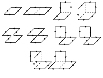
Figure 3: Wilson loops used in making the smeared glueball operators.

What we obtain from the MC simulation are the $24\times 24$ correlation matrix

$$\tilde{C}_{\alpha\beta}(t)=\sum\limits_{\tau}\langle 0|\bar{\phi}_{\alpha}^{(R)}(t+\tau)\bar{\phi}_{\beta}^{(R)}(\tau)|0\rangle,$$ (23)

where the vacuum subtraction

$$\bar{\phi}_{\alpha}^{(R)}(t)=\phi_{\alpha}^{(R)}(t)-\langle 0|\phi_{\alpha}^{(R)}(t)|0\rangle$$ (24)

is only applied to the $A_{1}^{++}$ channel which has a vacuum expectation value. The coefficients are determined in the data analysis stage by minimizing the effective mass

$$\tilde{m}(t_{D})=-\frac{1}{t_{D}}\ln\frac{\sum\limits_{\alpha\beta}v_{\alpha}^{(R)}v_{\beta}^{(R)}\tilde{C}_{\alpha\beta}(t_{D})}{\sum\limits_{\alpha\beta}v_{\alpha}^{(R)}v_{\beta}^{(R)}\tilde{C}_{\alpha\beta}(0)},$$ (25)

where the time separation for optimization is fixed to $t_{D}=1$. This is equivalent to solving the generalized eigenvalue equation

$$\tilde{C}(t_{D}){\bf v}^{(R)}=e^{-t_{D}\tilde{m}(t_{D})}\tilde{C}(0){\bf v}^{(R)}.$$ (26)

and the eigenvector ${\bf v}_{0}^{(R)}$, corresponding to the lowest effective mass $\tilde{m}_{0}(t_{D})$, yields the coefficients $v_{0\alpha}^{(R)}$ for the operator $O_{S}^{(R)}(t)$ which, under ordinary circumstances, best overlaps with the lowest-lying glueball $G_{0}$ in the channel of interest. The operators most overlapping with the excited states can also be constructed accordingly.

After the smeared operators are determined, the glueball masses and the matrix elements we are concerned with can be extracted by fitting two two-point functions, namely, the smeared-smeared correlation function,

$$C_{SS}(t) = \sum\limits_{\tau}\langle 0|O_{S}(t+\tau)O_{S}(\tau)|0\rangle$$ (27)

$$= \sum\limits_{n}\frac{1}{2M_{n}V}\langle 0|O_{S}|n\rangle\langle n|O_{S}|0\rangle e^{-m_{n}t}$$

$$\sim \frac{1}{2m_{G}V}|\langle G|O_{S}|0\rangle|^{2}e^{-M_{G}t}~{}~{}(t\rightarrow\infty),$$

and the smeared-local one

$$C_{SL}(t) = \sum\limits_{\tau}\langle 0|O_{S}(t+\tau)O_{L}(\tau)|0\rangle$$

$$= \sum\limits_{n}\frac{1}{2M_{n}V}\langle 0|O_{S}|n\rangle\langle n|O_{L}|0\rangle e^{-m_{n}t}$$

$$\sim \frac{1}{2M_{G}V}\langle G|O_{S}|0\rangle\langle 0|O_{L}|G\rangle e^{-M_{G}t}~{}~{}(t\rightarrow\infty).$$

$C_{SS}(t)$ and $C_{SL}(t)$ can be fitted simultaneously with three parameters, i.e., $\langle 0|O_{S}|G\rangle$, $\langle 0|O_{L}|G\rangle$, and the ground state glueball mass $M_{G}$. $\langle 0|O_{L}|G\rangle$ is the glueball matrix element we would like to obtain. Of course, before the physical results can be derived, a proper renormalization scheme should be performed.

In the following, we describe the calculation details step by step.

A. Setting the Scale Using the Static Potential

Table 5: The lattice spacings determined by $r_{0}^{-1}=410(20)$ MeV at different $\beta$.

$\beta$	$r_{0}/a_{s}$	$a_{s}/r_{0}$	$a_{s}$ (fm)
2.4	2.17(1)	0.461(2)	0.222(1)
2.6	2.74(2)	0.365(2)	0.176(1)
2.7	3.09(2)	0.326(2)	0.156(1)
3.0	4.05(4)	0.247(2)	0.119(1)
3.2	4.76(5)	0.210(2)	0.101(1)

The five lattice spacings $a_{s}$ are determined by calculating the heavy quark static potential. This part of the calculation is independent of the production runs. The static-quark potential $V({\bf r})$ can be extracted from the averages of Wilson loops $W({\bf r},t)$,

$$W({\bf r},t)=Z({\bf r})\exp(-tV({\bf r}))+\ldots$$ (29)

which can be measured precisely on the lattice. For each $\beta$, 200 configurations are generated, each of which is separated by 30 compound sweeps so that the auto-correlation effects are reduced. Secondly, these configuration are fixed to temporal gauge so that the Wilson loops can be calculated more easily. Different smearing schemes are applied to Wilson loops with different size to increase the overlapping with the ground states. Finally, the static potential is fitted by the model

$$V({\bf r})=V_{0}+\sigma r+\frac{e_{c}}{r},$$ (30)

with three parameters $V_{0}$, $\sigma$, and $e_{c}$ in the correlated fit method. The lattice spacing $a_{s}$ is determined by

$$\frac{a_{s}}{r_{0}}=\sqrt{\frac{\sigma a_{s}^{2}}{1.65+e_{c}}},$$ (31)

according to the relation $r^{2}dV({\bf r})/dr]_{r=r_{0}}=1.65$, where $r_{0}$ is hadronic scale parameter sommer94 . The lattice spacings for different $\beta$ are listed in Table 5.

B. The Glueball Mass Spectrum

Glueball masses can be obtained by fitting the two-point functions $C_{SS}(t)$ directly. It is taken as a testimony of the effectiveness of the improvement and smearing scheme old3 . Even though we are interested in the glueball matrix elements of the four channels $A_{1}^{++}$, $A_{1}^{-+}$, $E^{++}$, and $T_{2}^{++}$ in this work, glueball masses of all the 20 channels $R^{PC}$ are calculated as a by-product.

After the implementation of variational-optimization in each channel, we can obtain a specific operator which overlaps most with the a specific state and has little contaminations from other states with the same $J^{PC}$, so that we can use a single mass term

$$C_{SS}(t)=Z\left(e^{-Mt}+e^{-M(T-t)}\right),$$ (32)

to fit the two-point function in a time range $t_{min},\ldots,t_{max}$, which can be determined by observing the effective mass plateau. As a convention in this work, we use $M_{G}$ to represent the mass of a glueball state in the physical units and $M$ to represent the dimensionless mass parameter in the data processing with the relation $M=M_{G}a_{t}$. Generally speaking, for most channels in each of the five $\beta$ cases, the overlap of the specific operators on the ground states are all larger than 90%.

Before performing the continuum extrapolation, we check the finite volume effects of glueball masses. Three independent calculations at $\beta=2.4$, $\xi=5$ were carried out on a $8^{3}\times 40$ lattice, a $12^{3}\times 64$, and a $16^{3}\times 80$ lattice. These lattices have spatial volumes of $(1.76~{}{\rm fm})^{3}$, $(2.64~{}{\rm fm})^{3}$, and $(3.52~{}{\rm fm})^{3}$, respectively, with the lattice spacing $a_{s}\sim 0.22\,{\rm fm}$ from $r_{0}^{-1}=410(20)$ MeV. For these three runs, all the input parameters are the same except the different lattice volume.

The calculated glueball mass spectra are listed in Table 6, where one can find at a glance that the finite volume effects are very small and in most case the changes are within errors and consistent with zero statistically. More precisely, we use the following scheme to illustrate the finite volume effect (FVE) quantitatively. Let $\bar{M}$ denote the average value of the glueball masses from the three lattice volumes, $M(L)$ denotes the glueball mass measured on lattice $L^{3}\times T$. The fractional change of the glueball mass is defined by $\delta_{G}(L)=1-M(L)/\bar{M}$. The results for these fractional changes are shown in Fig. 4. Each point in the figure shows the fractional change $\delta_{G}(L)$ of the glueball mass, the error bars come from the statistical errors of $M(L)$, the solid lines indicate $\delta_{G}=0$, the dotted lines above and below the solid lines indicate $\delta_{G}=0.02$ and $\delta_{G}=-0.02$, respectively. All changes are statistically consistent with zero, suggesting that systematic errors in these results from finite volume are no larger than the statistical errors for these physical volumes. Since the physical volumes of the other $\beta$ values are not smaller than the $8^{3}\times 40$ at $\beta=2.4$, we shall neglect the FVE for the higher $\beta$ results.

Table 6: The fitted ground state masses in the twenty $R^{PC}$ channels at $\beta=2.4$ and $\xi=5$ on three different lattices $L^{3}\times T=16^{3}\times 80$, $12^{3}\times 64$, and $8^{3}\times 40$.

	$L=16$	$L=12$	$L=8$
$A_{1}^{++}$	0.308(3)	0.308(2)	0.312(2)
$A_{1}^{+-}$	1.082(14)	1.051(13)	1.079(10)
$A_{1}^{-+}$	0.604(11)	0.618(4)	0.618(3)
$A_{1}^{--}$	1.03(3)	1.075(16)	1.01(3)
$A_{2}^{++}$	0.825(8)	0.818(8)	0.820(5)
$A_{2}^{+-}$	0.805(6)	0.804(8)	0.808(5)
$A_{2}^{-+}$	1.047(10)	1.067(12)	1.053(12)
$A_{2}^{--}$	0.993(11)	0.976(10)	0.994(27)
$E^{++}$	0.542(3)	0.536(2)	0.541(2)
$E^{+-}$	0.919(17)	0.957(8)	0.960(6)
$E^{-+}$	0.699(4)	0.698(4)	0.695(3)
$E^{--}$	0.879(5)	0.891(7)	0.882(5)
$T_{1}^{++}$	0.826(5)	0.832(4)	0.834(3)
$T_{1}^{+-}$	0.657(6)	0.661(5)	0.663(4)
$T_{1}^{-+}$	0.932(5)	0.940(5)	0.936(4)
$T_{1}^{--}$	0.865(12)	0.884(5)	0.893(4)
$T_{2}^{++}$	0.542(3)	0.536(3)	0.538(2)
$T_{2}^{+-}$	0.807(4)	0.808(11)	0.799(8)
$T_{2}^{-+}$	0.697(5)	0.700(4)	0.700(2)
$T_{2}^{--}$	0.903(4)	0.893(6)	0.896(3)

Figure 4: Finite-volume effects of glueball masses at $\beta=2.4$, $\xi=5$. Each point shows the fractional change $\delta_{G}(L)=1-M(L)/\bar{M}$ of the glueball mass, where $M(L)$ is the glueball mass measured on the lattice $L^{3}\times T$ with $L=8,12,$ and 16, and $\bar{M}$ is the average values over those from different lattices. The errorbars come from the statistical errors of $M(L)$. The lattice labels $L$ are shown along the horizontal axis, and the labels along the vertical axis are the irreps of lattice symmetry group. The solid lines indicates $\delta_{G}=0$, and the dotted lines above the solid lines indicates $\delta_{G}=0.02$, and the dotted line lines below the solid lines indicate $\delta_{G}=-0.02$.

The fitted glueball masses at different coupling constant $\beta$ are listed in Table 7, where the statistical errors are also quoted. The dimensionless products of $r_{0}$ and the glueball masses $M_{G}$ are shown as functions of $(a_{s}/r_{0})^{2}$. To remove discretization errors from our estimates, the results for each level in these figures must be extrapolated to the continuum limit $a_{s}/r_{0}\rightarrow 0$. From perturbation theory, the leading discretization errors are expected to be $O(a_{t}^{2},a_{s}^{4},\alpha_{s}a_{s}^{2})$. As discussed in Ref. old3 , the $O(a_{t}^{2},\alpha_{s}a_{s}^{2})$ errors could be negligible compared to the $O(a_{s}^{4})$ errors for most calculated glueball masses except for $A_{1}^{++}$ glueball, so the fit model for these glueball masses is chosen to be

$$M_{G}(a_{s})r_{0}=M_{G}(0)r_{0}+c_{4}\frac{a_{s}^{4}}{r_{0}^{4}}.$$ (33)

The masses versus $(a_{s}/r_{0})^{2}$, as well as the fitted curves are shown in Fig. 5, 6, 7, and  8. One can find from the figures that the data obey this function very well. However, for $A_{1}^{++}$ glueball mass, the $O(a_{s}^{2})$ error seems still very large. So we keep the linear term of $a_{s}^{2}$ in the fit model, namely,

$$M_{G}(a_{s})r_{0}=M_{G}(0)r_{0}+c_{2}\frac{a_{s}^{2}}{r_{0}^{2}}+c_{4}\frac{a_{s}^{4}}{r_{0}^{4}}.$$ (34)

Already there has been some discussion on the possible reason for this large discretization error in scalar channel; one can refer to Ref. old3 for details.

We list several continuum extrapolated glueball masses in Table 8. We note that the earlier work old3 was carried out with $\beta=1.7,1.9,2.2,2,4,2.5$ and 3.0. In the present work, we concentrate on finer lattice spacings with $\beta=2.4,2.6,2.7,3.0$ and 3.2. For comparison, we have listed the results from the previous work old3 .

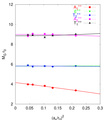
Figure 5: Masses of $PC=++$ glueballs in terms of $r_{0}$ against the lattice spacing square $(a_{s}/r_{0})^{2}$. The calculated values are plotted in points, and the curves are the best fits.

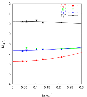
Figure 6: Masses of $PC=-+$ glueballs in terms of $r_{0}$ against the lattice spacing square $(a_{s}/r_{0})^{2}$. The calculated values are plotted in points, and the curves are the best fits.

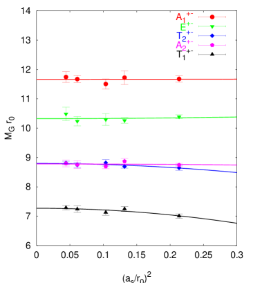
Figure 7: Masses of $PC=+-$ glueballs in terms of $r_{0}$ against the lattice spacing square $(a_{s}/r_{0})^{2}$. The calculated values are plotted in points, and the curves are the best fits.

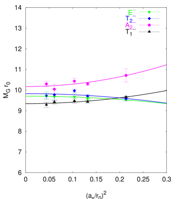
Figure 8: Masses of $PC=--$ glueballs in terms of $r_{0}$ against the lattice spacing square $(a_{s}/r_{0})^{2}$. The calculated values are plotted in points, and the curves are the best fits.

Table 7: The fitted ground state masses $M$ in the twenty $R^{PC}$ channels at five different $\beta$’s. The errors quoted here are all statistical errors from correlated minimal-$\chi^{2}$ method.

$R^{PC}$	$\beta=2.4$	$\beta=2.6$	$\beta=2.7$	$\beta=3.0$	$\beta=3.2$
$A_{1}^{++}$	0.312(2)	0.264(2)	0.247(2)	0.325(3)	0.279(5)
$A_{1}^{+-}$	1.079(10)	0.851(17)	0.741(11)	0.961(10)	0.822(13)
$A_{1}^{-+}$	0.618(3)	0.470(4)	0.410(3)	0.515(6)	0.439(4)
$A_{1}^{--}$	1.01(3)	0.897(20)	0.815(5)	1.036(12)	0.879(19)
$A_{2}^{++}$	0.820(5)	0.665(4)	0.593(6)	0.779(17)	0.683(17)
$A_{2}^{+-}$	0.808(5)	0.644(7)	0.560(5)	0.721(11)	0.616(8)
$A_{2}^{-+}$	1.053(12)	0.850(7)	0.745(26)	1.02(4)	0.868(18)
$A_{2}^{--}$	0.994(27)	0.748(5)	0.672(9)	0.827(21)	0.721(9)
$E^{++}$	0.541(2)	0.418(2)	0.374(3)	0.475(5)	0.414(4)
$E^{+-}$	0.960(6)	0.745(7)	0.663(13)	0.843(13)	0.734(16)
$E^{-+}$	0.695(3)	0.543(4)	0.486(3)	0.627(3)	0.514(3)
$E^{--}$	0.882(5)	0.695(6)	0.623(10)	0.797(29)	0.682(13)
$T_{1}^{++}$	0.834(3)	0.645(5)	0.561(3)	0.736(8)	0.628(4)
$T_{1}^{+-}$	0.663(4)	0.526(6)	0.459(6)	0.596(9)	0.510(5)
$T_{1}^{-+}$	0.936(4)	0.737(7)	0.664(9)	0.844(11)	0.714(6)
$T_{1}^{--}$	0.893(4)	0.685(5)	0.610(7)	0.776(8)	0.650(9)
$T_{2}^{++}$	0.538(2)	0.419(2)	0.375(4)	0.476(8)	0.413(5)
$T_{2}^{+-}$	0.799(8)	0.631(4)	0.568(7)	0.720(7)	0.617(4)
$T_{2}^{-+}$	0.700(2)	0.540(3)	0.479(4)	0.604(10)	0.510(3)
$T_{2}^{--}$	0.896(3)	0.705(5)	0.642(5)	0.805(23)	0.680(10)

Table 8: Continuum-limit glueball masses $M_{G}$. The corresponding results in Reference old3 are also quoted for comparison.

$R^{PC}$	Possible $J^{PC}$	$r_{0}M_{G}$ (this work)	$r_{0}M_{G}$ old3
$A_{1}^{++}$	$0^{++}$	4.16(11)	4.21(11)
$E^{++}$	$2^{++}$	5.82(5)	5.85(2)
$T_{2}^{++}$	$2^{++}$	5.83(4)	5.85(2)
$A_{2}^{++}$	$3^{++}$	9.00(8)	8.99(4)
$T_{1}^{++}$	$3^{++}$	8.87(8)	8.99(4)
$A_{1}^{-+}$	$0^{-+}$	6.25(6)	6.33(7)
$T_{1}^{+-}$	$1^{+-}$	7.27(4)	7.18(3)
$E^{-+}$	$2^{-+}$	7.49(7)	7.55(3)
$T_{2}^{-+}$	$2^{-+}$	7.34(11)	7.55(3)
$T_{2}^{+-}$	$3^{+-}$	8.80(3)	8.66(4)
$A_{2}^{+-}$	$3^{+-}$	8.78(5)	8.66(3)
$T_{1}^{--}$	$1^{--}$	9.34(4)	9.50(4)
$E^{--}$	$2^{--}$	9.71(3)	9.59(4)
$T_{2}^{--}$	$2^{--}$	9.83(8)	9.59(4)
$A_{2}^{--}$	$3^{--}$	10.25(4)	10.06(21)
$E^{+-}$	$2^{+-}$	10.32(7)	10.10(7)
$A_{1}^{+-}$	$0^{+-}$	11.66(7)	11.57(12)

C. The Glueball Matrix Elements

Figure 9: The effective mass plateaus of the smeared-smeared and smeared-local correlation functions at $\beta=2.4,\xi=5$ on the lattice $8^{3}\times 40$. The smeared-local correlation functions are plotted on the negative-time side of the $t$ axis. The Type-I local operators are used.

Figure 10: The effective mass plateaus of the smeared-smeared and smeared-local correlation functions at $\beta=2.4,\xi=5$ on the lattice $8^{3}\times 40$. The smeared-local correlation functions are plotted on the negative-time side of the $t$ axis. The Type-II local operators are used.

As described above, we use the correlated minimal-$\chi^{2}$ method to fit the smeared-smeared and smeared-local two-point functions, namely, $C_{SS}(t)$ and $C_{SL}(t)$, simultaneously using the fit functions

$$C_{SS}(t) = X^{2}\left(e^{-Mt}+e^{-M(T-t)}\right)$$

$$C_{SL}(t) = XY\left(e^{-Mt}+e^{-M(T-t)}\right),$$ (35)

where $X=\langle 0|O_{S}(0)|G\rangle/\sqrt{2M_{G}V}$ and $Y=\langle 0|O_{L}(0)|G\rangle/\sqrt{2M_{G}V}$. Here $V$ is the spatial lattice volume in physical units, say, $V=L^{3}a_{s}^{3}$, and $M_{G}=Ma_{t}^{-1}$. As an example, we show the effective mass plot at $\beta=2.4$ ($L=8$ lattice) in Figs. 9, and  10, where the smeared-local correlation functions are plotted on the negative-time side of the $t$ axis. In each channel, the effective mass plateau for $C_{SS}$ are flatter than that of $C_{SL}$. Nevertheless, both of them can be fitted by the same mass parameter consistently. For all the five $\beta$’s, the fit parameters $X$,$Y$, effective masses $M$, as well as the fit windows, are listed in Table 9, 10, 11, 12, and 13. In these tables, the first group of data is for Type-I operators, the second group for Type-II operators, and the last two row of data for the second definition (Eq. (II)) of Type-II operators in $T_{2}$ irreps. We give a brief interpretation of the meaning of the value of $X$ parameter here. During the practical performance of the variational method discussed in Sec. III, the eigenvectors ${\bf v}^{(R)}$ in Eq. (26) are normalized as ${{\bf v}^{(R)}}^{T}\tilde{C}(0){\bf v}^{(R)}=1$, so that the parameter $X$ indicates the relative overlap of the smeared operator to the specific stationary state (the ground state here). In these tables, all the $X$ parameters are very close to 1 which implies that the smeared operators couple almost completely to the ground state and there is little contamination from excited states. The $\chi^{2}$’s per degree of freedom of the data fitting are all acceptable and also listed in the tables.

Table 9: The matrix elements extracted at $\beta=2.4$ (on lattice $8^{3}\times 40$). The smeared-smeared(SS) and smeared-local(SL) correlators are fitted simultaneously in the time window $t$(SS) and $t$(SL). The fitted masses $M$, $X$, and $Y$ parameters are listed. The first group of data is for Type-I operators, the second group for Type-II operators, and the last two row of data for the second definition (Eq. (II)) of Type-II operators in $T_{2}$ irreps.

R	$t$(SS)	$t$(SL)	$M$	$Y$(${}\times 10^{-2}$)	$X$	$\chi^{2}/d.o.f$
$(S,B)$	1 – 4	1 – 3	0.311(2)	21.3(1)	0.994(3)	0.92
$(S,E)$	1 – 4	1 – 4	0.311(2)	21.1(2)	0.994(3)	0.69
$(PS)$	1 – 5	2 – 4	0.617(4)	5.24(11)	0.985(4)	1.59
$(E,B)$	1 – 7	1 – 5	0.541(2)	2.64(3)	0.995(2)	0.64
$(E,E)$	1 – 7	1 – 4	0.541(2)	1.52(9)	0.995(2)	0.64
$(T_{2},B)$	2 – 7	1 – 4	0.539(3)	1.84(12)	0.989(2)	0.57
$(T_{2},E)$	2 – 7	1 – 3	0.539(3)	0.85(5)	0.990(2)	0.52
$(S,B)$	1 – 9	1 – 7	0.311(2)	11.54(6)	0.993(3)	1.12
$(S,E)$	1 – 9	1 – 7	0.311(2)	16.38(13)	0.995(3)	0.75
$(PS)$	2 – 7	1 – 6	0.617(4)	5.33(11)	0.985(4)	1.36
$(E,B)$	1 – 7	1 – 6	0.541(2)	2.50(2)	0.995(2)	0.89
$(E,E)$	1 – 7	1 – 3	0.542(2)	1.35(4)	0.995(2)	0.87
$(T_{2},B)$	2 – 7	1 – 5	0.541(2)	2.24(1)	0.990(3)	1.34
$(T_{2},E)$	2 – 7	2 – 4	0.542(2)	0.73(4)	0.989(2)	0.45
$(T_{2},B)$	2 – 7	2 – 5	0.543(2)	2.37(1)	0.990(2)	1.06
$(T_{2},E)$	2 – 7	1 – 4	0.542(2)	0.73(4)	0.989(2)	0.46

Table 10: The same as in Table 9, but for $\beta=2.6$

R	$t$(SS)	$t$(SL)	$M$	$Y$(${}\times 10^{-2}$)	$X$	$\chi^{2}/d.o.f$
$(S,B)$	1 – 9	1 – 7	0.264(2)	6.48(5)	0.994(3)	0.92
$(S,E)$	1 – 9	1 – 7	0.264(2)	6.37(11)	0.994(3)	0.69
$(PS)$	2 – 7	1 – 5	0.470(4)	2.14(3)	0.985(4)	1.59
$(E,B)$	1 – 7	1 – 6	0.424(2)	0.716(10)	0.995(2)	0.64
$(E,E)$	1 – 7	1 – 3	0.423(2)	0.39(4)	0.995(2)	0.64
$(T_{2},B)$	2 – 7	1 – 5	0.421(1)	0.562(7)	0.989(2)	0.57
$(T_{2},E)$	2 – 7	1 – 4	0.421(2)	0.23(2)	0.990(2)	0.52
$(S,B)$	1 – 9	1 – 7	0.265(2)	4.01(3)	0.993(3)	1.12
$(S,E)$	1 – 9	1 – 7	0.263(2)	5.06(3)	0.995(3)	0.75
$(PS)$	2 – 7	1 – 6	0.470(5)	2.16(3)	0.985(4)	1.36
$(E,B)$	1 – 7	1 – 6	0.424(2)	0.706(13)	0.995(2)	0.89
$(E,E)$	1 – 7	1 – 3	0.424(2)	0.40(3)	0.995(2)	0.87
$(T_{2},B)$	2 – 7	1 – 5	0.423(2)	0.698(5)	0.990(3)	1.34
$(T_{2},E)$	2 – 7	2 – 4	0.421(2)	0.22(2)	0.989(2)	0.45
$(T_{2},B)$	2 – 7	2 – 5	0.422(2)	0.719(10)	0.990(2)	1.06
$(T_{2},E)$	2 – 7	1 – 4	0.421(2)	0.22(2)	0.989(2)	0.46

Table 11: The same as in Table 9, but for $\beta=2.7$

R	$t$(SS)	$t$(SL)	$M$	$Y$(${}\times 10^{-2}$)	$X$	$\chi^{2}/d.o.f$
$(S,B)$	2 – 9	1 – 7	0.247(2)	5.03(4)	0.990(3)	0.92
$(S,E)$	2 – 9	1 – 7	0.246(2)	4.88(13)	0.991(3)	0.50
$(PS)$	1 – 7	2 – 6	0.431(3)	1.88(5)	0.991(2)	1.07
$(E,B)$	3 – 8	1 – 4	0.376(3)	0.575(10)	0.982(4)	0.75
$(E,E)$	3 – 8	1 – 3	0.376(4)	0.27(3)	0.981(4)	0.39
$(T_{2},B)$	4 – 8	2 – 6	0.379(5)	0.423(10)	0.977(7)	1.14
$(T_{2},E)$	4 – 8	1 – 4	0.378(6)	0.20(2)	0.975(8)	1.39
$(S,B)$	2 – 9	3 – 7	0.246(2)	3.21(4)	0.990(3)	0.86
$(S,E)$	2 – 9	3 – 7	0.247(2)	3.80(10)	0.990(3)	0.58
$(PS)$	2 – 7	1 – 6	0.431(2)	1.90(5)	0.991(2)	1.08
$(E,B)$	3 – 8	2 – 5	0.376(3)	0.592(10)	0.981(4)	0.60
$(E,E)$	3 – 8	2 – 5	0.376(3)	0.27(2)	0.982(4)	0.22
$(T_{2},B)$	4 – 8	2 – 6	0.386(5)	0.546(10)	0.988(8)	1.79
$(T_{2},E)$	4 – 8	1 – 3	0.378(5)	0.19(2)	0.975(8)	1.28
$(T_{2},B)$	4 – 8	3 – 6	0.386(5)	0.565(9)	0.987(8)	1.82
$(T_{2},E)$	4 – 8	2 – 3	0.378(5)	0.19(2)	0.975(8)	1.29

Table 12: The same as in Table 9, but for $\beta=3.0$

R	$t$(SS)	$t$(SL)	$M$	$Y$(${}\times 10^{-2}$)	$X$	$\chi^{2}/d.o.f$
$(S,B)$	2 – 9	1 – 4	0.324(3)	1.56(3)	0.985(3)	0.99
$(S,E)$	2 – 9	1 – 4	0.326(4)	1.50(4)	0.985(3)	0.82
$(PS)$	2 – 5	1 – 4	0.542(6)	0.706(15)	0.981(6)	2.00
$(E,B)$	3 – 7	1 – 4	0.480(6)	0.176(7)	0.967(8)	0.22
$(E,E)$	3 – 7	1 – 3	0.480(6)	0.107(14)	0.967(8)	0.25
$(T_{2},B)$	3 – 8	1 – 3	0.487(5)	0.137(5)	0.969(7)	1.28
$(T_{2},E)$	3 – 8	1 – 3	0.485(6)	0.060(9)	0.967(7)	0.94
$(S,B)$	2 – 9	2 – 7	0.326(4)	1.07(2)	0.984(3)	0.68
$(S,E)$	2 – 9	1 – 8	0.324(3)	1.09(3)	0.986(3)	0.49
$(PS)$	2 – 5	1 – 4	0.541(6)	0.715(15)	0.981(5)	1.84
$(E,B)$	3 – 7	1 – 4	0.477(6)	0.179(5)	0.964(8)	0.72
$(E,E)$	3 – 7	1 – 3	0.480(6)	0.086(5)	0.967(8)	0.22
$(T_{2},B)$	3 – 8	1 – 4	0.490(5)	0.172(4)	0.971(7)	1.55
$(T_{2},E)$	3 – 8	1 – 3	0.485(6)	0.053(6)	0.968(8)	1.17
$(T_{2},B)$	3 – 8	1 – 4	0.489(5)	0.179(4)	0.971(7)	1.46
$(T_{2},E)$	3 – 8	1 – 3	0.485(6)	0.053(6)	0.968(8)	1.17

Table 13: The same as in Table 9, but for $\beta=3.2$

R	$t$(SS)	$t$(SL)	$M$	$Y$(${}\times 10^{-2}$)	$X$	$\chi^{2}/d.o.f$
$(S,B)$	4 – 7	1 – 6	0.279(6)	0.518(11)	0.966(9)	1.74
$(S,E)$	4 – 7	1 – 4	0.278(5)	0.534(26)	0.965(9)	0.18
$(PS)$	3 – 9	3 – 6	0.439(8)	0.294(15)	0.932(9)	0.38
$(E,B)$	3 – 7	1 – 4	0.417(4)	0.062(4)	0.967(3)	2.77
$(E,E)$	3 – 7	1 – 3	0.415(4)	0.048(8)	0.965(3)	1.49
$(T_{2},B)$	3 – 9	1 – 4	0.414(3)	0.0548(13)	0.959(4)	0.67
$(T_{2},E)$	3 – 9	1 – 3	0.415(3)	0.033(5)	0.960(5)	0.67
$(S,B)$	4 – 7	1 – 8	0.282(5)	0.391(7)	0.968(7)	1.98
$(S,E)$	4 – 7	1 – 6	0.280(5)	0.376(11)	0.967(8)	0.31
$(PS)$	3 – 9	3 – 6	0.439(8)	0.299(15)	0.932(9)	0.40
$(E,B)$	3 – 7	1 – 3	0.415(4)	0.0693(23)	0.966(4)	3.29
$(E,E)$	3 – 7	1 – 3	0.416(4)	0.037(4)	0.965(4)	3.05
$(T_{2},B)$	3 – 9	1 – 7	0.416(4)	0.068(2)	0.961(6)	0.96
$(T_{2},E)$	3 – 9	1 – 3	0.415(3)	0.028(3)	0.960(4)	0.56
$(T_{2},B)$	3 - 9	2 - 5	0.415(4)	0.068(3)	0.960(5)	0.74
$(T_{2},B)$	3 - 9	1 - 3	0.415(3)	0.028(3)	0.960(4)	0.54

From the measured matrix elements of the two definitions of the Type-II local operators in tensor channel ($T_{2}$ irreps), we can get an estimate of the $O(a_{s}^{4})$ lattice artifacts. Recalling the discussion in Sec. II, after restoring the fact $ig$ to $F_{\mu\nu}$, the difference of the two definition of the operators $(T_{2},B)$ is

$$\Delta=\frac{1}{36}a_{s}^{8}g^{2}(D_{\mu}^{2}+D_{\nu}^{2})F_{\mu\nu}(D_{\rho}^{2}+D_{\sigma}^{2})F_{\rho\sigma}+\ldots,$$ (36)

with the indices $\mu$, $\nu$, $\rho$, and $\sigma$ varying accordingly. The ratio of the matrix elements of the two definitions of operator $(T_{2},B)$ is plotted in Fig. 11 with respect to the lattice spacing. It is known that this difference comes totally from the lattice discretization and will disappear in the continuum limit. This is the case from the figure. Even though the relative difference is less than 3–4%, the deviation of the ratio from 1 is detectable on coarse lattice with larger lattice spacing and decreases when approaching to the continuum limit. On the finest lattice we are using, the difference is consistent with zero within the error. This result shows that, as far as the Type-II operators are concerned, after the implementation of Symanzik’s improvement scheme along with the tadpole improvement, the measured matrix elements of the two versions of lattice local operator have a few percent differences at finite $a_{s}$, but approaches the same continuum limit as $a_{s}$ goes to zero.

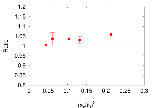
Figure 11: The data points represent the ratios of the matrix elements of the two definitions of operator $(T_{2},B)$ at different lattice spacings. The straight line is plotted to show how far the ratios deviate from 1.

Here comes the discussion of the FVE of the matrix elements. By analogy with the FVE analysis of glueball masses, the glueball matrix elements are also calculated at $\beta=2.4$ and $\xi=5$ on a $8^{3}\times 40$ lattice, a $12^{3}\times 64$, and a $16^{3}\times 80$ lattice. For these three runs, all the input parameters are the same except the different lattice volume. The extracted matrix elements are listed in Table 14, 15, and 16, respectively for Type-I and Type-II operators. As illustrated in the tables, the finite volume effects of matrix elements are very small and in most case the changes are consistent with zero statistically. We also define the relative deviation $\delta_{G}(L)=1-f_{G}(L)/\bar{f}_{G}$ to show the FVE quantitatively, where $\bar{f}_{G}$ is the mean value of the matrix elements of glueball $G$ averaged over the three lattice volumes, $f_{G}(L)$ denote the matrix element of glueball $G$ measured on lattice $L^{3}\times T$. The results of $\delta_{G}(L)$ are shown in Fig. 12. In the figure, each point shows $\delta_{G}(L)$ of the matrix element of a glueball $G$, and the error bars come from the statistical errors of $f_{G}(L)$. The solid lines indicates $\delta_{G}=0$, the dotted lines above and below the solid lines indicate $\delta_{G}=\pm 0.02$. The largest effects from the finite volume appear to occur in the TYPE I operator of $(E,B)$. All deviations are statistically consistent with zero, suggesting that systematic errors in these results from finite volume are no larger than the statistical errors. Since the physical volumes of the other $\beta$ values are not smaller than the $8^{3}\times 40$ at $\beta=2.4$, we shall neglect the finite volume effects for the higher $\beta$ results.

Table 14: The finite volume effects of matrix elements at $\beta=2.4$ and $\xi=5$ on three different lattices $L^{3}\times T=16^{3}\times 80$, $12^{3}\times 64$, and $8^{3}\times 40$. The fitted $Y$ parameters are listed in normal numbers. For clarity, the $Y$ parameters for lattice $L=12$ and $L=8$ are re-scaled to $L=16$ due to the relation $Y=\langle 0|O_{L}(0)|G\rangle/\sqrt{2M_{G}V}$ and illustrated by bold numbers. This table lists the $Y$ parameters of Type-I operators.

	$L=16$	$L=12$	$L=8$
$(S,B)$	7.53(5)	7.50(5)	7.52(5)
	7.53(5)	11.54(7)	21.27(15)
$(S,E)$	7.38(12)	7.51(11)	7.47(8)
	7.38(12)	11.56(17)	21.12(23)
$(E,B)$	0.956(12)	0.993(8)	0.936(11)
	0.956(12)	1.53(12)	2.64(3)
$(E,E)$	0.56(5)	0.52(4)	0.54(3)
	0.56(5)	0.81(6)	1.52(9)
$(T_{2},B)$	0.633(8)	0.649(8)	0.651(4)
	0.633(8)	1.000(12)	1.841(11)
$(T_{2},E)$	0.29(2)	0.27(3)	0.30(2)
	0.29(2)	0.42(4)	0.85(6)
$(PS)$	1.85(4)	1.88(4)	1.85(4)
	1.85(4)	2.89(6)	5.24(11)

Table 15: The same as Table 14, but for Type-II operators.

	$L=16$	$L=12$	$L=8$
$(S,B)$	0.410(3)	0.408(3)	0.408(2)
	4.10(3)	6.29(4)	11.54(6)
$(S,E)$	5.73(6)	5.82(4)	0.579(4)
	5.73(6)	8.97(6)	16.4(1)
$(E,B)$	0.885(11)	0.895(9)	0.883(7)
	0.885(11)	1.378(14)	2.50(2)
$(E,E)$	47(2)	0.47(2)	0.48(2)
	0.47(2)	0.72(3)	1.35(4)
$(T_{2},B)$	0.783(5)	0.792(4)	0.790(4)
	0.783(5)	1.220(6)	2.24(1)
$(T_{2},E)$	0.25(2)	0.26(2)	0.26(2)
	0.25(2)	0.40(3)	0.73(4)
$(PS)$	1.87(4)	1.90(4)	1.89(4)
	1.87(4)	2.92(6)	5.33(11)

Table 16: The same as Table 14, but for the second definition of Type-II operators $O(T_{2},B)$ and $O(T_{2},E)$.

	$L=16$	$L=12$	$L=8$
$(T_{2},B)$	0.825(6)	0.835(8)	0.837(4)
	0.825(6)	1.285(12)	2.367(12)
$(T_{2},E)$	0.26(2)	0.26(2)	0.26(2)
	0.26(2)	0.40(3)	0.73(4)

Figure 12: Finite-volume effects on the results of the $\beta=2.4$, $\xi=5$ calculation. Each point shows the fractional change $\delta_{G}(L)=1-f_{G}(L)/\bar{f}_{G}$ in the matrix element of a glueball $G$, where $f_{G}(L)$ is the matrix element of $G$ measured on the lattice $L^{3}\times T$ with $L=8,12,$ and 16, and $\bar{f}_{G}$ is the average values over those from different lattices. The errorbars come from the statistical errors of $f_{G}(L)$. The lattice labels $L$ are shown along the horizontal axis, and the labels of different local operators are specified along the vertical axis. The solid lines indicates $\delta_{G}=0$, and the dotted lines above the solid lines indicates $\delta_{G}=0.02$, and the dotted line lines below the solid lines indicate $\delta_{G}=-0.02$. The FVE of different definitions of local operators are also shown in the figure.

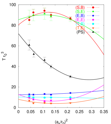
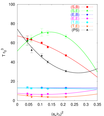
Figure 13: Glueball matrix elements(ME) in terms of $r_{0}^{3}$ against the lattice spacing square $(a_{s}/r_{0})^{2}$. The calculated values of ME’s are plotted in points, with different colors corresponding to different channels. The curves are best fits to the calculated results by the model $T(a_{s})r_{0}^{3}=T(0)r_{0}^{3}+c_{2}(a_{s}/r_{0})^{2}+c_{4}(a_{s}/r_{0})^{4}$. The left panel illustrates the result of Type-I operators, while the right panel is for Type-II operators.

Based on the discussions above, in the following continuum extrapolation of matrix elements, we use the results calculated on the lattice $8^{3}\times 40$ at $\beta=2.4$. As for the Type-II operators, we take the results with the lattice operators defined by $\hat{F}_{\mu\nu}(x)\hat{F}_{\rho\sigma}(x)$

Using the fitted $M$ and $Y$ parameters listed in Table 9-13, as well as the physical values of the lattice spacings $a_{s}$ listed in Table 5 for each $\beta$, the lattice matrix elements $\langle 0|O_{L}|G\rangle$ can be obtained by $\langle 0|O_{L}|G\rangle=\sqrt{2M_{G}V}Y$. As a result, the matrix elements in units of $r_{0}^{-3}$ are listed in Table 17 and illustrated by Figure 13.

Table 17: Final results of matrix elements of lattice gluonic operators. The data in table are in the unit of $r_{0}^{-3}$ with $r_{0}^{-1}=0.410(20)\,{\rm MeV}$.

	$\beta=2.4$	$\beta=2.6$	$\beta=2.7$	$\beta=3.0$	$\beta=3.2$
	($L=8$)	($L=12$)	($L=12$)	($L=16$)	($L=24$)
$T(S,B)_{I}$	87(2)	90(2)	94(3)	92(3)	85(4)
$T(S,E)_{I}$	86(2)	89(4)	91(6)	90(6)	88(7)
$T(E,B)_{I}$	14.2(3)	12.5(5)	13.2(7)	12.6(8)	12.8(10)
$T(E,E)_{I}$	8.2(6)	6.8(10)	6.2(9)	7.9(12)	9.6(22)
$T(T_{2},B)_{I}$	9.9(3)	9.8(4)	9.7(5)	9.8(7)	11.0(6)
$T(T_{2},E)_{I}$	4.5(4)	4.1(6)	4.6(8)	4.3(7)	6.7(14)
$T(PS)_{I}$	30(1)	40(2)	46(3)	52(3)	61(5)
$T(S,B)_{II}$	47(1)	56(1)	60(2)	63(2)	64(3)
$T(S,E)_{II}$	67(2)	70(2)	71(4)	65(4)	62(4)
$T(E,B)_{II}$	13.4(4)	12.3(4)	13.6(5)	12.8(8)	13.8(9)
$T(E,E)_{II}$	7.3(3)	7.0(7)	6.2(6)	6.2(6)	7.4(10)
$T(T_{2},B)_{II}$	12.7(3)	12.6(5)	13.0(7)	12.8(7)	13.6(9)
$T(T_{2},E)_{II}$	3.9(3)	3.8(5)	4.4(5)	3.8(6)	5.6(10)
$T(PS)_{II}$	31(1)	40(2)	47(2)	53(3)	62(5)

It is clear that the continuum limits can be extrapolated neither by the function with a single $a_{s}^{2}$ term nor with a single $a_{s}^{4}$ term. We fit them with the form

$$T(a_{s})r_{0}^{3}=T(0)r_{0}^{3}+c_{2}\frac{a_{s}^{2}}{r_{0}^{2}}+c_{4}\frac{a_{s}^{4}}{r_{0}^{4}},$$ (37)

where $T$ is the final non-renormalized continuum limit results of the glueball matrix elements.

Note that these matrix elements are all calculated by bare lattice operators. Before the renormalization of the local operators is performed, we cannot draw any conclusions of physical interest at present stage. However, we can give some comments on the different behaviors of the matrix elements of the Type-I and Type-II operators from the continuum extrapolation. Based on our experience from the calculation of glueball masses, the continuum $SO(3)$ symmetry is approximately restored for all the lattice spacings we use in this work, since the calculated glueball masses in $T_{2}^{++}$ and $E^{++}$ channel are coincident. The left panel of Fig. 13 is the plot of the matrix elements of the Type-I operators, where one can find that the calculated glueball matrix elements of $T_{2}$ and $E$ irreps do not show this symmetry restoration. This is probably due to the definition of the Type-I operator introduced in Sec. II. The Type-I operators with different quantum number are defined by the real part of different Wilson loops composed of different numbers of spatial gauge links, such that the overall tadpole improvement factors (different powers of the tadpole parameter $u_{s}$) are different for $T_{2}$ and $E$ representation. The conjectured power counting of the tadpole parameter $u_{s}$ for Wilson loops is a naive approximation and may bring additional deviation to the local operators. We have carried out the test that the naive tadpole parameters are replaced by the vacuum expectation value (VEV) of the corresponding Wilson loops. As we expected, the two matrix elements tend to coincide better. In contrast with the Type-I operators, all the Type-II operators are defined by the improved lattice version of the gauge strength tensor, $\hat{F}_{\mu\nu}$, and thus have the same correction factor coming from the tadpole improvement. The right panel of Fig. 13 shows the behaviors of the matrix elements of the Type-II operators. It is clearly seen that the approximate $SO(3)$ symmetry restoration takes place for $T_{2}$ and $E$ representation.

The matrix elements of phenomenological interest, denoted $s$, $p$ and $t$, are defined as

$$(2\pi)^{3}\delta(\bf{0})s = \langle 0|\int d^{3}xS(x)|G\rangle,$$

$$(2\pi)^{3}\delta(\bf{0})p = \langle 0|\int d^{3}xP(x)|G\rangle,$$

$$(2\pi)^{3}\delta(\bf{0})t\epsilon_{\mu\nu} = \langle 0|\int d^{3}x\Theta_{\mu\nu}(x)|G\rangle,$$ (38)

where $\epsilon_{\mu\nu}=\epsilon_{\nu\mu}$, $\epsilon_{\mu\mu}=0$, $\epsilon_{\mu\nu}\epsilon_{\mu\nu}=1$, and $S(x)$, $P(x)$, $\Theta_{\mu\nu}(x)$ are defined in Eq. (II) and Eq. (II). Recalling that $(2\pi)^{3}\delta(\bf{0})$ is replaced by $L^{3}a_{s}^{3}$ on finite lattices, and combining Eq. (II-II), $s$, $p$, and $t$ can be reproduced by the calculated matrix elements listed in Table 17 as

$$sr_{0}^{3} = 2(T(S,B)+T(S,E)),$$

$$pr_{0}^{3} = 8T(PS),$$

$$t_{E}r_{0}^{3} = 2|T(E,B)-T(E,E)|,$$

$$t_{T_{2}}r_{0}^{3} = 2|T(T_{2},B)-T(T_{2},E)|.$$ (39)

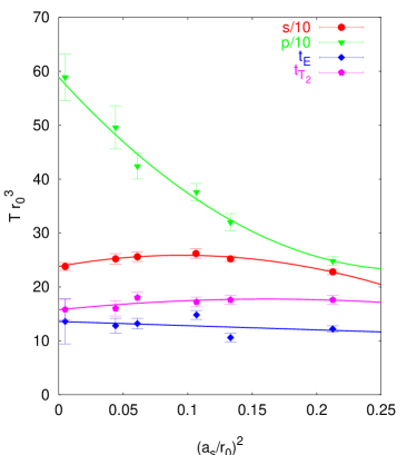
Figure 14: The non-renormalized matrix elements $s$, $p$ and $t$ from type-II operators are plotted versus lattice spacing. The continuum extrapolations are also carried out.

Fig. 14 and Table 18 illustrate the behaviors of these matrix elements with respect to the lattice spacings. We only show the data reproduced from the Type-II operators, which can be only renormalized in this work (see Section V). The continuum limits of $t_{T_{2}}$ and $t_{E}$ are consistent within error bars. The deviation of the central values comes mainly from the discrepancy of $T(E,E)$ and $T(T_{2},E)$.

Table 18: The non-renormalized matrix elements $s$, $p$, and $t$ in units of $r_{0}^{-3}$ are reproduced from the lattice results of type-II operators at different lattice spacings. The errors quoted here are purely statistical. The continuum limits are also listed for each channel.

	$\beta=2.4$	$\beta=2.6$	$\beta=2.7$	$\beta=3.0$	$\beta=3.2$	Continuum
$sr_{0}^{3}$	228(5)	252(5)	262(9)	256(9)	252(10)	227(7)
$pr_{0}^{3}$	248(8)	320(16)	376(16)	424(24)	496(40)	589(43)
$t_{E}r_{0}^{3}$	12.2(5)	10.6(8)	14.8(8)	13.2(1.0)	12.8(1.4)	13.6(4.1)
$t_{T_{2}}r_{0}^{3}$	17.6(0.8)	17.6(0.8)	17.2(0.9)	18.0(1.0)	16.0(1.4)	15.8(1.9)

V. The Non-Perturbative Renormalization of Local Gluonic Operators

The lattice local gluonic operator $O$ and its continuum counterpart $O_{cont}$ is related by the renormalization constant $Z_{O}(a)$,

$$O_{cont}=a^{-4}Z_{O}(a)O.$$ (40)

The key question is to choose a proper normalization condition, so that the renormalization constant can be determined. In this work, we choose the energy-momentum tensor in the glueball state as the normalization condition.

The energy-momentum tensor for the pure gauge theory

$$\bar{T}_{\mu\nu}=\bar{T}_{\nu\mu}=-\frac{1}{2}\delta_{\mu\nu}{\rm Tr}F^{2}+2{\rm Tr}F_{\mu\alpha}F_{\nu\alpha}$$ (41)

satisfies $\partial_{\mu}\bar{T}_{\mu\nu}=0$ and does not need an overall renormalization in the continuum. More specifically, $\bar{T}_{00}=Tr({\bf E}^{2}-{\bf B}^{2})$). At the classical level, $\bar{T}_{\mu\nu}$ is traceless. When quantum corrections are included, the renormalized energy-momentum tensor, $T_{\mu\nu}$, takes a non-vanishing trace part, $\hat{T}_{\mu\nu}$, which comes from the anomalous breaking of scale invariance and is called the QCD trace anomaly,

$$\hat{T}_{\mu\nu}=-\frac{1}{4}\frac{\beta(g)}{2g}\delta_{\mu\nu}F^{2}=\frac{11}{32\pi^{2}}\delta_{\mu\nu}Tr(g^{2}{\bf B}^{2}+g^{2}{\bf E}^{2}),$$ (42)

where $\beta(g)=-\beta_{0}g^{3}/(4\pi)^{2}$ is the $\beta$ function of QCD to the lowest order of the coupling constant $g$ with $\beta_{0}=11$ in the pure gauge case. Thus, $T_{\mu\nu}$ can be written explicitly as the sum of the traceless and trace parts,

$$T_{\mu\nu}=\bar{T}_{\mu\nu}+\hat{T}_{\mu\nu}.$$ (43)

On the other hand, $T_{\mu\nu}$ defines the Hamiltonian operator of the theory

$$H=\int d^{3}xT_{00}({\bf x},0),$$ (44)

which is finite and scale independent. In the rest frame of a glueball, the matrix element of the Hamiltonian $H$ in the glueball state is just the glueball’s rest mass,

$$M_{G}=\frac{\langle G(M_{G},{\bf p}=0)|\int d^{3}xT_{00}({\bf x},0)|G(M_{G},{\bf p}=0)\rangle}{\langle G|G\rangle}.$$ (45)

If the glueball states $|G(E,{\bf p})\rangle$ are normalized as

$$\langle G(E_{p},{\bf p})|G(E_{p},{\bf p^{\prime}})\rangle=2E_{p}(2\pi)^{3}\delta^{3}({\bf p}-{\bf p^{\prime}}),$$ (46)

we have $\langle G(M_{G},{\bf p}=0)|\int d^{3}xT_{00}({\bf x},0)|G(M_{G},{\bf p}=0)\rangle=2M_{G}^{2}(2\pi)^{3}\delta^{3}({\bf 0})\equiv 2p^{0}p^{0}(2\pi)^{3}\delta^{3}({\bf 0})$, which implies that

$$\langle G(p)|\int d^{3}xT_{\mu\nu}({\bf x},0)|G(p)\rangle=2p^{\mu}p^{\nu}(2\pi)^{3}\delta^{3}({\bf 0}).$$ (47)

Combining Eq. (45) and (47), we get the normalization conditions in the glueball’s rest frame,

$$\langle G(p)|\int d^{3}x\bar{T}_{\mu\nu}({\bf x},0)|G(p)\rangle = 2(p^{\mu}p^{\nu}-\frac{1}{4}M_{G}^{2}\delta_{\mu\nu})(2\pi)^{3}\delta^{3}({\bf 0}),$$

$$\langle G(p)|\int d^{3}x\hat{T}_{\mu\nu}({\bf x},0)|G(p)\rangle = \frac{1}{2}M_{G}^{2}\delta_{\mu\nu}(2\pi)^{3}\delta^{3}({\bf 0}).$$

According to the definitions in Eq. II and Eq. II, the $E$ and $T_{2}$ operators are related to $\bar{T}_{ij}$ by

$$O_{1}^{(E,E)}-O_{1}^{(E,B)} \propto \bar{T}_{11}-{\bar{T}}_{22},$$

$$O_{2}^{(E,E)}-O_{2}^{(E,B)} \propto 2{\bar{T}}_{33}-\bar{T}_{11}-\bar{T}_{22},$$

$$O_{i}^{(T_{2},E)}-O_{i}^{(T_{2},B)} \propto \epsilon_{ijk}\bar{T}_{jk},$$ (49)

whose matrix elements in a zero-momentum glueball state vanish, thus we cannot renormalize $E^{++}$ and $T_{2}^{++}$ operators directly by the normalization condition in Eq. V. The Non-Perturbative Renormalization of Local Gluonic Operators in the glueball rest frame. A possible way around this difficulty is to assume the almost restoration of Lorentz invariance at the lattice spacings we use in this work, so the overall renormalization constant of the lattice version of $\bar{T}_{\mu\nu}$ can be determined by one of its components. In fact, this is justified to some extent by two facts. First, it is argued that the rotational invariance can be restored if the scale parameter $z=m_{A_{1}^{++}}L$ is larger than 10 lusher , and our smallest lattice gives the value $z=0.31\times 5\times 8=12.4$ which meets this requirement. Secondly, in our lattice calculations of the mass spectrum and matrix elements, the coincidence of $E^{++}$ channel and $T_{2}^{++}$ channel implies that this rotational restoration is actually realized. Based on the discussion above, we choose the component $\bar{T}_{00}$ to do the renormalization of the tensor operator in this work. In the practical study, we calculate the matrix elements $\langle G|O_{\pm}|G\rangle_{\rm lat}$, where $O_{\pm}$ is the operator $g^{2}Tr({\bf E}^{2}\pm{\bf B}^{2})$ and $|G\rangle=|A_{1}^{++}\rangle$, $|E^{++}\rangle$, or $|T_{2}^{++}\rangle$. As we have addressed before, $O_{-}$ is proportional to $\bar{T}_{00}$, and $O_{+}$ is proportional to the trace anomaly $\hat{T}_{00}$. Thus, the renormalization constants of the scalar and tensor operators can be extracted from these matrix elements.

The matrix elements $\langle G|O_{\pm}|G\rangle_{\rm lat}$ can be obtained by calculating the three-point function

$$C_{3}(t_{1},t_{2}) = \langle 0|O_{s}(-t_{1})O_{\pm}(0)O_{s}(t_{2})|0\rangle=\sum\limits_{m,n}\frac{1}{4E_{n}E_{m}V^{2}}\langle 0|O_{S}(-t_{1})|n\rangle\langle n|O_{\pm}(0)|m\rangle\langle m|O_{S}(t_{2})|0\rangle$$ (50)

$$= \sum\limits_{m,n}\frac{1}{4E_{n}E_{m}V^{2}}\langle 0|O_{S}(0)|n\rangle\langle n|O_{\pm}(0)|m\rangle\langle m|O_{S}(0)|0\rangle e^{-E_{n}t_{1}}e^{-E_{m}t_{2}}$$

$$\rightarrow \frac{1}{(2M_{G}V)^{2}}\langle 0|O_{s}(0)|G\rangle|^{2}\langle G|O_{\pm}(0)|G\rangle e^{-M_{G}(t_{1}+t_{2})}~{}~{}(t_{1},~{}t_{2}\rightarrow\infty)$$

where $O_{S}(t)$ is the smeared zero-momentum operator which generates the ground state $|G\rangle$ from the vacuum, and $M_{G}$ the ground state mass. Using the asymptotic form of the two-point function

$$C_{SS}(t)\sim\frac{1}{2M_{G}V}|\langle 0|O_{S}(0)|G\rangle|^{2}e^{-M_{G}t}~{}~{}(t\rightarrow\infty)$$ (51)

and dividing the three-point function by proper two-point function, one gets

$$\frac{C_{3}(t_{1},t_{2})}{C_{SS}(t_{1})}\approx\frac{1}{2M_{G}V}\langle G|O_{\pm}(0)|G\rangle e^{-M_{G}t_{2}}~{}~{}(t_{1},t_{2}\rightarrow\infty).$$ (52)

In the practical data processing, by analogy with the extraction of the matrix element, we fit $C_{2}(t)$ and $C_{3}(t,t_{0})$ simultaneously with the fitting model

$$C_{SS}(t) = X^{2}e^{-Mt}$$

$$C_{3}(t,t_{0}) = X^{2}We^{-M(t+t_{0})},$$ (53)

where $t_{0}=1$. $W$ is related to the matrix element $\langle G|O_{\pm}(0)|G\rangle$ by

$$\langle G|O_{\pm}(0)|G\rangle=2M_{G}VW.$$ (54)

From Eq. (40), Eq. (V. The Non-Perturbative Renormalization of Local Gluonic Operators) and the fitted matrix elements $\langle G|O_{\pm}|G\rangle_{\rm lat}$, the renormalization constants for scalar and tensor gluonic operators can be derived as

$$\frac{1}{Z_{S}(a_{s})} = \frac{11}{32\pi^{2}}\frac{2}{M_{G}^{2}a_{s}^{4}}\langle G|O_{+}|G\rangle_{\rm lat},$$

$$\frac{1}{Z_{T}(a_{s})} = \frac{1}{g^{2}}\frac{2}{3M_{G}^{2}a_{s}^{4}}\langle G|O_{-}|G\rangle_{\rm lat},$$ (55)

where the coupling constant $g^{2}$ comes from the relation $\bar{T}_{00}=(1/g^{2})O_{-}$.

Unfortunately, the gluonic three-point function is far more noisy than the gluonic two-point function in Monte Carlo calculation. In this work, the renormalization of gluonic operators is performed only at $\beta=2.4$ on the lattice $8^{3}\times 40$ with $\xi=5$. As many as 100,000 measurements are carried out, the signals of three point functions are still weak with large fluctuation. In the practical computation, the matrix elements of Type-I and Type-II operators of $O^{(S,B)}$ and $O^{(S,E)}$ are all calculated. It is found that the three-point functions involving Type-I operators are so noisy that the matrix elements cannot be extracted reliably. The three-point functions involving Type-II operators behave better, from which we obtain the renormalization constants. The matrix elements $\langle G|O_{\pm}|G\rangle_{\rm lat}$ and the resultant renormalization constants at $\beta=2.4$ are listed in Table 19.

Table 19: The matrix elements of operator $O_{\pm}$ (Type-II) in glueball states are listed. $S$ represents the scalar glueball state, while $T(E)$ and $T(T_{2})$ denotes the tensor glueballs in $E$ and $T_{2}$ irreps, respectively. The renormalization constants extracted from these matrix elements are given also.

$|G\rangle$	$\langle G|O_{+}|G\rangle_{\rm lat}$	$Z_{S}$	$\langle G|O_{-}|G\rangle_{\rm lat}$	$Z_{T}$
$S$	32(9)	1.1(3)	13(5)	0.7(3)
$T(E)$	102(16)	1.0(2)	51(15)	0.53(15)
$T(T_{2})$	101(16)	1.0(2)	53(15)	0.51(15)

Table 20: The non-renormalized topological susceptibility $\chi_{L}(a_{s})$ calculated at different lattice spacing are listed in physical units. Also listed are the ratios of $\chi_{L}^{1/2}(a_{s})$ and the non-renormalized matrix elements of pseudoscalar $p(a_{s})$ after rescaled by their continuum extrapolation values $\chi_{L}^{1/2}(0)$ and $p(0)$.

$\beta$	2.4	2.6	2.7	3.0	3.2	continuum
$\chi_{L}^{1/4}(a_{s})({\rm MeV})$	242(4)	277(5)	299(5)	323(6)	351(8)	391(15)
$p(a_{s})r_{0}^{3}$	248(8)	320(16)	376(16)	424(24)	496(40)	589(43)
$\frac{p(a_{s})\chi_{L}^{1/2}(0)}{\chi_{L}^{1/2}(a_{s})p(0)}$	1.10(7)	1.08(9)	1.09(8)	1.06(10)	1.05(11)	1.00(13)

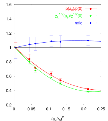
Figure 15: The $a_{s}$-dependences of $\chi_{L}^{1/2}(a_{s})$ and $p(a_{s})$ are plotted. For comparison, $\chi_{L}^{1/2}(a_{s})$ and $p(a_{s})$ are rescaled by their continuum-extrapolated values, say, $\chi_{L}^{1/2}(0)$ and $p(0)$, respectively. One can find that the $a_{s}$-dependences of $\chi_{L}^{1/2}(a_{s})$ and $pr_{0}^{3}(a_{s})$ are very similar and their ratios are fairly constant.

As for the renormalization of the pseudoscalar operator, we tentatively use the phenomenological value of the topological susceptibility, $\chi^{1/4}=180\,{\rm MeV}$, as the normalization condition. The quantity $\chi$ is defined by

$$\chi=\int d^{4}x\langle q(x)q(0)\rangle,$$ (56)

where the topological charge density $q(x)$ is proportional to the pseudoscalar operator $P(x)$ (defined in Eq. (II) as $q(x)=\frac{1}{32\pi^{2}}P(x)$. The lattice version of $\chi$, denoted by $\chi_{L}$, is defined by the lattice pseudoscalar operator $O(PS)(x)$ as

$$\chi_{L}=\frac{\xi}{(32\pi^{2})^{2}L^{3}Ta_{s}^{4}}\sum\limits_{x,y}\langle O^{(PS)}(x)O^{(PS)}(y)\rangle,$$ (57)

where $L$ and $T$ are the lattice sizes in spatial and temporal directions, respectively.

We have calculated $\chi_{L}(a_{s})$ for all the five $\beta$, at each $\beta$ 20000 measurements are carried out. In Table 20 are listed the results of $\chi_{L}^{1/4}(a_{s})$ in units of MeV for different $\beta$, as well as the non-renormalized continuum value $\chi_{L}^{1/4}(0)$ after the continuum extrapolation $a_{s}\rightarrow 0$. It is obvious that the value of $\chi_{L}^{1/4}(a_{s})$ increases along with the decreasing of lattice spacing. For comparison, the non-renormalized matrix elements $pr_{0}^{3}(a_{s})$ at different $\beta$’s are also listed in Table 20. In Fig. 15 are plotted the $a_{s}$-dependences of $\chi_{L}^{1/2}(a_{s})$ and $pr_{0}^{3}(a_{s})$ (rescaled by their continuum-extrapolated values, respectively), as well as their ratios, where one can find that the $a_{s}$-dependences of $\chi_{L}^{1/2}(a_{s})$ and $pr_{0}^{3}(a_{s})$ are very similar and their ratios are fairly constant. Using $\chi^{1/4}=180\,{\rm MeV}$, the renormalization constant $Z_{P}$ of pseudoscalar operator in the continuum limit can be extracted as

$$Z_{P}=\frac{\chi^{1/2}}{\chi_{L}^{1/2}(0)}\approx 0.21(2)$$ (58)

VI. RESULTS AND DISCUSSION

After the continuum extrapolation and the renormalization of the local operators, we can discuss the physical implication of our lattice results.

As we addressed above, we have tried to extract the renormalization constants for scalar and tensor operator only at $\beta=2.4$. In fact, the signals of the three-point functions of type-I operator are very poor, so the renormalization constants $Z_{S}$ and $Z_{T}$ are obtained only for Type-II operators. We are lucky with this situation because all the Type-II operators are made up of the lattice version of the gauge field strength, $\hat{F}_{\mu\nu}$, thus they all have the same normalization constant, say, the same tadpole-improvement factor. Therefore, for Type-II operator, the $Z_{T}$ extracted from $\bar{T}_{00}$ can be applied to other components involved in the glueball matrix elements calculated in this work.

Considering Eq. (II) and (6), the non-renormalized matrix elements of the $S(x)$, $P(x)$, and $\Theta(x)$ in the continuum can be obtained by the lattice results, and are shown in Table 18. We notice that, although the $(S,B)$ and $(S,E)$ matrix elements have sizeable $a_{s}$ dependence for the Type-II operator, as seen in Fig. 13, the total scalar matrix element, which is the sum of the two, is much flatter in $(a_{s}/r_{0})^{2}$. This is also the case for the tensor matrix element. With the observation that the non-renormalized matrix elements of the scalar and the tensor depend on the lattice spacing $(a_{s}/r_{0})^{2}$ very mildly, we speculate that there is not a large lattice spacing dependence in the renormalization constant, and will use $Z_{S}$ and $Z_{T}$ computed at $\beta=2.4$ as an approximation of the renormalization constants in the continuum limit. We shall check this in the future when computer resources are available for high statistics calculation at larger $\beta$.

Taking the average of the renormalization constant $Z_{S}$ from Table 19, we get a continuum extrapolated value for the matrix element $\langle 0|S|0^{++}\rangle=15.6\pm 3.2\,{\rm GeV}^{3}$. Based on the scaling properties of QCD and trace anomaly, both the QCD sum rule sumrule and the soft meson theorem softmeson lead to an estimate that relates the scalar glueball matrix element to the gluon condensate,

$$\langle 0|S|0^{++}\rangle=16\pi^{2}\sqrt{\frac{G_{0}}{2b}}M_{G},$$ (59)

where $G_{0}=\langle 0|\frac{\alpha_{s}}{\pi}G_{\mu\nu}^{a}G_{\mu\nu}^{a}|0\rangle$ is the gluon condensate, $b=(11/3)N_{c}-(2/3)N_{f}$ and $M_{G}$ the scalar glueball mass. Taking $N_{f}=0$, $G_{0}=0.012\,{\rm GeV}^{4}$, and $M_{G}\approx 1.7\,{\rm GeV}$, this matrix element is estimated to be $\sim 6.3$ GeV, which is about two and a half times smaller than our lattice result. This discrepancy might be attributable to the fact that the quenched lattice calculation gives a gluon condensate which is about $0.14\pm 0.02{\rm GeV}^{4}$ giacomo . This is larger by an order of magnitude than that used in QCD sum rule. If the relation Eq. (59) still holds in the pure gauge theory, using the quenched gluon condensate, the estimated scalar matrix element is estimate to be $(21\pm 1){\rm GeV}^{3}$ which is in good agreement with our quenched lattice calculation.

For the pseudoscalar, with the renormalization constant $Z_{P}=0.21(2)$ determined in last section, the lattice calculation gives the result $\langle 0|P|0^{-+}\rangle\approx 8.6\pm 1.3\,{\rm GeV}^{3}$. It has been proposed that there is an approximate chiral symmetry between the scalar and pseudoscalar glueballs chiral . A sum rule is derived from an effective action which relates the topological susceptibility $\chi$ in the pure gauge case to the gluon condensate $G_{0}$,

$$\chi=\eta^{-2}\sqrt{\frac{G_{0}}{2b}},$$ (60)

where $\eta\approx 0.7$. Using our lattice results, the degree of chiral symmetry $\eta$ can be obtained from the ratio of the pseudoscalar to scalar matrix elements chiral , $\eta_{L}=\langle 0|P|0^{-+}\rangle/(2\langle 0|S|0^{++}\rangle)\approx 0.3$, which is also more than two times smaller than the result of QCD sum rule. These facts hint that there may be a substantial quenching effect in the matrix element of the scalar.

We can also estimate the glueball contribution to the topological susceptibility by the lattice matrix element and glueball mass,

$$\chi_{\rm glueball}=\left(\frac{\langle 0|P|0^{-+}\rangle}{32\pi^{2}M_{0^{-+}}}\right)^{2}\approx(103\,{\rm MeV})^{4}\sim 0.11\chi,$$ (61)

which implies that the pseudoscalar glueball gives an appreciable 11% contribution to the topological susceptibility.

In the tensor channel, the glueball matrix element is extrapolated to $1.0\pm 0.2\,{\rm GeV}^{3}$ in the continuum, which is the average of results of $E$ and $T_{2}$ channels. In the calculation, it is found that in the lattice spacing range we use, the glueball mass and matrix elements are approximately independent of the lattice spacing, this implies that the lattice artifacts might be neglected here. If the renormalization constant $Z_{T}\approx 0.52(15)$ of the tensor operator does not change much in the range of lattice spacing and applies to all the $\beta$ values in this work, the renormalized matrix element of tensor operator is $0.52\pm 0.19\,{\rm GeV}^{3}$, which is in agreement with the prediction $0.35\,{\rm GeV}^{3}$ from the tensor dominance model tensor and QCD sum rule sum3 for the tensor mass around $2.2\,{\rm GeV}$.

Table 21: The final glueball spectrum in physical units. In column 2, the first error is the statistical uncertainty coming from the continuum extrapolation, the second one is the 1% uncertainty resulting from the approximate anisotropy. In column 3, the first error comes from the combined uncertainty of $r_{0}M_{G}$, the second from the uncertainty of $r_{0}^{-1}=410(20)\,{\rm MeV}$

$J^{PC}$	$r_{0}M_{G}$	$M_{G}\,({\rm MeV}$)
$0^{++}$	4.16(11)(4)	1710(50)(80)
$2^{++}$	5.83(5)(6)	2390(30)(120)
$0^{-+}$	6.25(6)(6)	2560(35)(120)
$1^{+-}$	7.27(4)(7)	2980(30)(140)
$2^{-+}$	7.42(7)(7)	3040(40)(150)
$3^{+-}$	8.79(3)(9)	3600(40)(170)
$3^{++}$	8.94(6)(9)	3670(50)(180)
$1^{--}$	9.34(4)(9)	3830(40)(190)
$2^{--}$	9.77(4)(10)	4010(45)(200)
$3^{--}$	10.25(4))(10)	4200(45)(200)
$2^{+-}$	10.32(7)(10)	4230(50)(200)
$0^{+-}$	11.66(7)(12)	4780(60)(230)

VII. Conclusion

The glueball mass spectrum and glueball-to-vacuum matrix elements are calculated on anisotropic lattices in this work. The calculations are carried out at five lattice spacings $a_{s}$’s which range from $0.22\,{\rm fm}$ to $0.10\,{\rm fm}$. Due to the implementation of the improved gauge action and improved gluonic local operators, the lattice artifacts are highly reduced. The finite volume effects are carefully studied with the result that they can be neglected on the lattices we used in this work.

As to the glueball spectrum, we have carried out calculations similar to the previous work old3 on much larger and finer lattices, so that the liability of the continuum limit extrapolation is reinforced. Our results of the glueball spectrum is summarized in Tab. 21 and Fig. 16.

After the non-perturbative renormalization of the local gluonic operators, we finally get the matrix elements of scalar($s$), pseudoscalar($p$), and tensor operator ($t$) with the results

$$s = 15.6\pm 3.2~{}({\rm GeV})^{3}$$

$$p = 8.6\pm 1.3~{}({\rm GeV})^{3}$$

$$t = 0.52\pm 0.19~{}({\rm GeV})^{3},$$ (62)

where the errors of $s$ and $t$ come mainly from the errors of the renormalization constants $Z_{S}$ and $Z_{T}$. The more precise calculation of $Z_{S}$ and $Z_{T}$ will be carried out in later work.

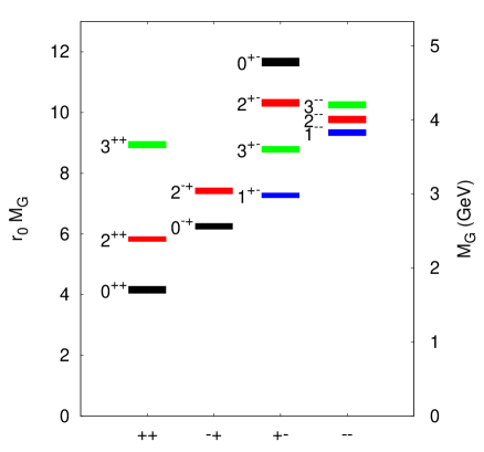
Figure 16: The mass spectrum of glueballs in the pure $SU(3)$ gauge theory. The masses are given both in terms of $r_{0}$ ($r_{0}^{-1}=410\,{\rm MeV}$) and in ${\rm GeV}$. The height of each colored box indicates the statistical uncertainty of the mass.

- (1) B. Berg and A. Billoire, Nucl. Phys. B221, 109 (1983).
- (2) G. Bali, et al. (UKQCD Collaboration), Phys. Lett. B 309, 378 (1993).
- (3) C. Michael and M. Teper, Nucl. Phys. B314, 347 (1989).
- (4) C. Morningstar and M. Peardon, Phys. Rev. D56, 3043 (1997); Phys. Rev. D60, 034509 (1999).
- (5) G.P. Lepage and P.B. Mackenzie, Phys. Rev. D48, 2250 (1993).
- (6) R. Sommer, Nucl. Phys. B411, 839 (1994).
- (7) K.F. Liu, B.A. Li, and K. Ishikawa, Phys. Rev. D40, 3648 (1989).
- (8) Y. Liang, K.F. Liu, B.A. Li, S.J. Dong, and K. Ishikawa, Phys. Lett. B307, 375 (1993).
- (9) X. Ji, Phys. Rev. Lett. 74, 1071 (1995).
- (10) M. Lüscher, Phys. Lett. 118B, 387 (1982).
- (11) S.J. Dong, et al., Nucl. Phys. Proc. Suppl. 63, 254 (1998).
- (12) Yu.A. Simonov, Phys. Atom. Nucl. 50, 213, (1989).
- (13) V.A. Novikov, M.A. Shifman, A.I. Vainshtein, and Zakharov, Nucl. Phys. B165, 67 (1980).
- (14) J. Ellis and J. Lanik, Phys. Lett. 150B, 289 (1985).
- (15) A.Di. Giacomo, H.G. Dosch, V.I. Shevchenko, Yu.A. Simonov, Phys. Rept. 372, 319 (2002), hep-lat/0007223.
- (16) J.M. Cornwall and A. Soni, Phys. Rev. D29 1424 (1984).
- (17) K. Ishikawa, I. Tanaka, K.F. Liu, and B.A. Li, Phys. Rev. D37, 3216 (1988).
- (18) S. Narison, Z. Phys. C26, 209 (1984).