The axial charge of the nucleon on the lattice and in chiral perturbation theory

Abstract:

We present recent Monte Carlo data for the axial charge of the nucleon obtained by the QCDSF-UKQCD collaboration for $N_{f}=2$ dynamical quarks. We compare them with formulae from chiral perturbation theory in finite and infinite volume and find a remarkably consistent picture.

PoS(LAT2005)349

The QCDSF and UKQCD collaborations have generated ensembles of gauge field configurations using $N_{f}=2$ non-perturbatively $O(a)$ improved Wilson quarks and Wilson’s plaquette action for the gauge fields. Here we want to discuss the results obtained for the axial charge of the nucleon, $g_{A}$. Their interpretation is not straightforward because the quark masses in the simulations are larger than in nature, the volumes are somewhat smaller than infinity, the lattice spacings are larger than 0 etc. So we need some guidance for the extrapolations towards the physical quark masses, the thermodynamic and continuum limits. Such guidance is provided by chiral effective field theory (ChEFT), which for selected quantities, e.g. for $g_{A}$, yields parameterisations of the dependence on the quark mass and the volume which take into account the constraints imposed by (spontaneously broken) chiral symmetry. The dependence on the lattice spacing $a$ can be included, but we shall not consider this possibility here. So we do not yet attempt to cope with the lattice artefacts remaining even after $O(a)$ improvement.

If ChEFT can be successfully applied, we gain control over the chiral extrapolation and the approach to the thermodynamic limit. At the same time we can determine not only the physical value of the quantity of interest, $g_{A}$ in our case, but also some effective coupling constants. These may occur in the ChEFT expressions for other observables and be of phenomenological interest there. Establishing the link between Monte Carlo results and ChEFT will thus enable us to extract considerably more information from our simulations than just the physical value of the quantity under study.

In its standard form, ChEFT describes low-energy QCD by means of an effective field theory based on effective pion, nucleon, … fields. Since the effective Lagrangian does not depend on the volume, besides the quark-mass dependence the very same Lagrangian governs also the volume dependence, and finite size effects can be calculated by evaluating the theory in a finite (spatial) volume. Thus the finite volume does not introduce any new parameters and the study of the finite size effects yields an additional handle on the coupling constants of ChEFT. The effective description will break down if the box length $L$ becomes too small, just as it fails for pion masses that are too large.

The simulation parameters are listed in Table 1. Note that we have two groups of three ensembles each which differ only in the volume.

Coll.	$\beta$	$\kappa_{\mathrm{sea}}$	volume
QCDSF	5.20	0.1342	$16^{3}\times 32$
UKQCD	5.20	0.1350	$16^{3}\times 32$
UKQCD	5.20	0.1355	$16^{3}\times 32$
QCDSF	5.25	0.1346	$16^{3}\times 32$
UKQCD	5.25	0.1352	$16^{3}\times 32$
QCDSF	5.25	0.13575	$24^{3}\times 48$
QCDSF	5.40	0.1350	$24^{3}\times 48$
QCDSF	5.40	0.1356	$24^{3}\times 48$
QCDSF	5.40	0.1361	$24^{3}\times 48$

Coll.	$\beta$	$\kappa_{\mathrm{sea}}$	volume
UKQCD	5.29	0.1340	$16^{3}\times 32$
QCDSF	5.29	0.1350	$16^{3}\times 32$
QCDSF	5.29	0.1355	$12^{3}\times 32$
QCDSF	5.29	0.1355	$16^{3}\times 32$
QCDSF	5.29	0.1355	$24^{3}\times 48$
QCDSF	5.29	0.1359	$12^{3}\times 32$
QCDSF	5.29	0.1359	$16^{3}\times 32$
QCDSF	5.29	0.1359	$24^{3}\times 48$

Table 1: Simulation parameters.

We compute $g_{A}$ from forward proton matrix elements of the flavour-nonsinglet axial vector current $A_{\mu}^{u-d}=\bar{u}\gamma_{\mu}\gamma_{5}u-\bar{d}\gamma_{\mu}\gamma_{5}d$:

$$\langle p,s|A_{\mu}^{u-d}|p,s\rangle=2g_{A}s_{\mu}\,.$$ (1)

The required bare matrix elements are extracted from ratios of 3-point functions over 2-point functions in the standard fashion. Compared to the computation of hadron masses, additional difficulties arise in the calculation of nucleon matrix elements such as $g_{A}$: In general there are quark-line disconnected contributions, which are hard to evaluate, the operators must be improved and renormalised etc. Fortunately, in the limit of exact isospin invariance, which is taken in our simulations, all disconnected contributions cancel in $g_{A}$, because it is a flavour-nonsinglet quantity. The improved axial vector current is given by

$$A_{\mu}^{\mathrm{imp}}(x)=\bar{q}(x)\gamma_{\mu}\gamma_{5}q(x)+ac_{A}\partial_{\mu}\bar{q}(x)\gamma_{5}q(x)\,,$$ (2)

and hence the improvement term, i.e. the term proportional to $c_{A}$, does not contribute in forward matrix elements. The renormalised improved axial vector current can be written as

$$A_{\mu}=Z_{A}\left(1+b_{A}am\right)A_{\mu}^{\mathrm{imp}}$$ (3)

with the bare quark mass $m=\left(1/\kappa_{\mathrm{sea}}-1/\kappa_{c}\right)/(2a)$.

While the coefficient $b_{A}$ will be computed in tadpole improved one-loop perturbation theory, we calculate the renormalisation factor $Z_{A}$ non-perturbatively by means of the Rome-Southampton method [1, 2]. Thus $Z_{A}$ is first obtained in the so-called RI’-MOM scheme. Using continuum perturbation theory we switch to the $\overline{\mbox{MS}}$ scheme. For sufficiently large renormalisation scales $\mu$, $Z_{A}$ should then be independent of $\mu$. However, unless $\mu\ll 1/a$ lattice artefacts may spoil this behaviour. Since our scales do not always satisfy this criterion, we try to correct for this mismatch by subtracting the lattice artefacts perturbatively with the help of boosted one-loop lattice perturbation theory. Some lattice artefacts still remain, but we can nevertheless estimate $Z_{A}$. In Table 2 we compare our results with a recent determination of $Z_{A}$ by the ALPHA collaboration [3].

$\beta$	5.20	5.25	5.29	5.40
this work	0.765(5)	0.769(4)	0.772(4)	0.783(4)
ALPHA	0.719	0.734	0.745	0.767

Table 2: Values of $Z_{A}$ from this work and from the ALPHA collaboration.

Our results for $g_{A}$ are plotted in Fig. 1. Here $m_{\pi}$ has been taken from the largest available lattice at each ($\beta$, $\kappa_{\mathrm{sea}}$) combination. The scale has been set by means of the force parameter $r_{0}$ with $r_{0}=0.467\,\mbox{fm}$, and $r_{0}/a$ has been taken at the given quark mass. Obviously there are considerable finite size effects. A similar volume dependence has already been observed in quenched simulations [4].

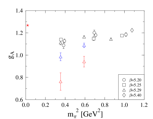
Figure 1: Results for $g_{A}$. The red triangles correspond to a spatial box length $L\approx 1.0\,\mbox{fm}$, the blue triangles belong to $L\approx 1.3\,\mbox{fm}$, and for the black symbols the volumes are larger. The red star represents the physical point.

In order to describe or fit these data we use ChEFT. More specifically, we employ the so-called small scale expansion (SSE) [5], which is one possibility to include explicit $\Delta$(1232) degrees of freedom in ChEFT. The small expansion parameter in the SSE is called $\epsilon$, and in $O(\epsilon^{3})$ the mass dependence of $g_{A}$ is given for infinite volume by [6]

$$\begin{array}[]{l}\displaystyle g_{A}^{SSE}(m_{\pi}^{2})=g_{A}^{0}+\left[4C^{HB}(\lambda)-\frac{(g_{A}^{0})^{3}}{16\pi^{2}F_{\pi}^{2}}-\frac{25c_{A}^{2}g_{1}}{324\pi^{2}F_{\pi}^{2}}+\frac{19c_{A}^{2}g_{A}^{0}}{108\pi^{2}F_{\pi}^{2}}\right]m_{\pi}^{2}\\[14.22636pt] \displaystyle{}-\frac{m_{\pi}^{2}}{4\pi^{2}F_{\pi}^{2}}\left[(g^{0}_{A})^{3}+\frac{1}{2}\,g^{0}_{A}\right]\ln{\frac{m_{\pi}}{\lambda}}+\frac{4c_{A}^{2}g_{A}^{0}}{27\pi\Delta_{0}F_{\pi}^{2}}\,m_{\pi}^{3}\\[14.22636pt] \displaystyle{}+\left[25c_{A}^{2}g_{1}\Delta_{0}^{2}-57c_{A}^{2}g_{A}^{0}\Delta_{0}^{2}-24c_{A}^{2}g_{A}^{0}m_{\pi}^{2}\right]\frac{\sqrt{m_{\pi}^{2}-\Delta_{0}^{2}}}{81\pi^{2}F_{\pi}^{2}\Delta_{0}}\arccos\frac{\Delta_{0}}{m_{\pi}}\\[14.22636pt] \displaystyle{}+\frac{25c_{A}^{2}g_{1}\left(2\Delta_{0}^{2}-m_{\pi}^{2}\right)}{162\pi^{2}F_{\pi}^{2}}\ln\frac{2\Delta_{0}}{m_{\pi}}+\frac{c_{A}^{2}g_{A}^{0}\left(3m_{\pi}^{2}-38\Delta_{0}^{2}\right)}{54\pi^{2}F_{\pi}^{2}}\ln\frac{2\Delta_{0}}{m_{\pi}}+O(\epsilon^{4})\,,\end{array}$$ (4)

where $g_{A}^{0}$ denotes the chiral limit value of $g_{A}$. This expression depends on several coupling constants, all referring to the chiral limit: $F_{\pi}$ is the pion decay constant with the physical value of about 92.4 MeV, $\Delta_{0}$ denotes the real part of the $N\Delta$ mass splitting, $c_{A}$ and $g_{1}$ are $N\Delta$ and $\Delta\Delta$ axial coupling constants, respectively. Finally, $C^{HB}(\lambda)$ is a counterterm at the renormalisation scale $\lambda$, which can be expressed in terms of the more conventional heavy-baryon couplings $B_{9}^{r}(\lambda)$ and $B_{20}^{r}(\lambda)$:

$$C^{HB}(\lambda)=B_{9}^{r}(\lambda)-2\,g_{A}^{0}B_{20}^{r}(\lambda)\,.$$ (5)

Evaluating the underlying ChEFT in a finite spatial volume yields an expression for the $L$ dependence of $g_{A}$ [7, 8].

Phenomenology provides some information on the parameters appearing above. The analysis of (inelastic) $\pi$ $N$ scattering, in particular the process $\pi N\to\pi\pi N$, suggests that choosing the physical pion mass as the scale $\lambda$ one has [6]

$$B_{9}^{r}(\lambda=m_{\pi}^{\mathrm{phys}})=(-1.4\pm 1.2)\,\mbox{GeV}^{-2}\quad,\quad B_{20}^{r}(\lambda=m_{\pi}^{\mathrm{phys}})\equiv 0\,.$$ (6)

Therefore we set $\lambda=0.14\,\mbox{GeV}$ in the following and identify $C^{HB}(\lambda=m_{\pi}^{\mathrm{phys}})=B_{9}^{r}(\lambda=m_{\pi}^{\mathrm{phys}})$. In the real world one has $\Delta_{0}=0.2711\,\mbox{GeV}$, and from an $O(\epsilon^{3})$ SSE analysis of the $\Delta$ width one finds $c_{A}=1.5$. At the physical pion mass we have $g_{A}=1.267$, while $g_{A}^{0}\approx 1.2$ [6]. Little is known about $g_{1}$. In the SU(6) quark model one finds $g_{1}=\frac{9}{5}g_{A}^{0}\approx\frac{9}{5}1.2=2.16$. For $F_{\pi}$ one expects in the chiral limit $F_{\pi}\approx 86.2\,\mbox{MeV}$.

Unfortunately, we cannot fit all parameters. So we fix $\Delta_{0}=0.2711\,\mbox{GeV}$, $c_{A}=1.5$, $F_{\pi}=86.2\,\mbox{MeV}$ and fit $g_{A}^{0}$, $B_{9}^{r}$, $g_{1}$ taking into account only pion masses below approximately 600 MeV. In contrast to Ref. [6] the physical point is not fitted. We find $g_{A}^{0}=1.15(12)$, $B_{9}^{r}=-0.71(18)\,\mbox{GeV}^{-2}$, $g_{1}=2.6(8)$ with $\chi^{2}/\mathrm{dof}=4.23/3$. Remarkably enough, these values are very well compatible with our phenomenological prejudices above. In Fig. 2 we plot the data with the finite size correction subtracted together with the fit curve. So, if the fit would be perfect the data points which differ only in the volume would collapse onto a single point.

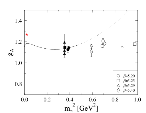
Figure 2: Results for $g_{A}$ with the finite size correction subtracted. The curve represents the first fit described in the text. The data points shown as open symbols have not been fitted.

The uncertainty in $g_{A}^{0}$ is large enough to cover the experimental point. To exemplify this circumstance we fix $g_{A}^{0}=1.225$, a value well within the range favoured by the above fit, and use only $B_{9}^{r}$ and $g_{1}$ as fit parameters. We find $B_{9}^{r}=-0.66(17)\,\mbox{GeV}^{-2}$ and $g_{1}=3.0(3)$ with $\chi^{2}/\mathrm{dof}=4.61/4$. In Fig. 3 we plot the data without subtracting the finite size corrections. Using the results of the last fit we show curves not only for $L=\infty$, but also for the values taken in the simulations for $\beta=5.29$, $\kappa_{\mathrm{sea}}=0.1359$. Of course, many more variations of the fit procedure are possible, but the overall pattern remains remarkably stable yielding $g_{A}^{0}\sim 1.2$, $B_{9}^{r}\sim-0.5\ldots-0.7\,\mbox{GeV}^{-2}$, $g_{1}\sim 3$ and $F_{\pi}\sim 90\,\mbox{MeV}$, in accordance with phenomenological expectations.

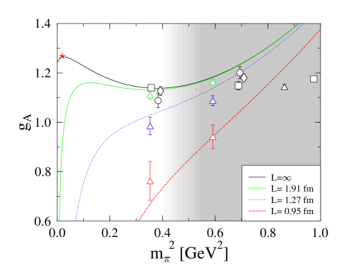
Figure 3: Results for $g_{A}$ with curves for several values of $L$.

References

- [1] G. Martinelli, C. Pittori, C. T. Sachrajda, M. Testa and A. Vladikas, A General method for nonperturbative renormalization of lattice operators, Nucl. Phys. B445 (1995) 81 [hep-lat/9411010].
- [2] M. Göckeler et al., Nonperturbative renormalisation of composite operators in lattice QCD, Nucl. Phys. B544 (1999) 699 [hep-lat/9807044].
- [3] M. Della Morte, R. Hoffmann, F. Knechtli, R. Sommer and U. Wolff, Non-perturbative renormalization of the axial current with dynamical Wilson fermions, JHEP 0507 (2005) 007 [hep-lat/0505026].
- [4] S. Sasaki, K. Orginos, S. Ohta and T. Blum, Nucleon axial charge from quenched lattice QCD with domain wall fermions, Phys. Rev. D68 (2003) 054509 [hep-lat/0306007].
- [5] T. R. Hemmert, B. R. Holstein and J. Kambor, Heavy baryon chiral perturbation theory with light deltas, J. Phys. G24 (1998) 1831 [hep-ph/9712496].
- [6] T. R. Hemmert, M. Procura and W. Weise, Quark mass dependence of the nucleon axial-vector coupling constant, Phys. Rev. D68 (2003) 075009 [hep-lat/0303002].
- [7] S. R. Beane and M. J. Savage, Baryon axial charge in a finite volume, Phys. Rev. D70 (2004) 074029 [hep-ph/0404131].
- [8] T. Wollenweber, Diploma Thesis, Technische Universität München (2005).
- [9] C. R. Allton et al. [UKQCD Collaboration], Effects of non-perturbatively improved dynamical fermions in QCD at fixed lattice spacing, Phys. Rev. D65 (2002) 054502 [hep-lat/0107021].