Determination of the spin-dependent potentials with the multi-level algorithm

Abstract:

The spin-dependent corrections to the static interquark potential are relevant to describing the fine and hyper-fine splittings of the heavy quarkonium spectra. We investigate these corrections in SU(3) lattice gauge theory with the Polyakov loop correlation function as the quark source by applying the multi-level algorithm. We observe remarkably clean signals for the spin-dependent potentials up to intermediate distances.

PoS(LAT2005)216

1 Introduction

The spin-dependent (spin-orbit, spin-spin) interquark potentials are relevant to describing the fine and hyper-fine splittings of the heavy quarkonium spectra and thus it is interesting to determine their behavior directly from QCD. Eichten and Feinberg [1] derived in this context the general form of the potential including the spin-dependent corrections up to $O(1/m^{2})$,

$$V(r) = V_{0}(r)+\left(\frac{\vec{s}_{1}\cdot\vec{l}_{1}}{2m_{1}^{2}}-\frac{\vec{s}_{2}\cdot\vec{l}_{2}}{2m_{2}^{2}}\right)\left(\frac{V_{0}^{\prime}(r)}{r}+2\frac{V_{1}^{\prime}(r)}{r}\right)+\left(\frac{\vec{s}_{2}\cdot\vec{l}_{1}}{2m_{1}m_{2}}+\frac{\vec{s}_{1}\cdot\vec{l}_{2}}{2m_{1}m_{2}}\right)\frac{V_{2}^{\prime}(r)}{r}$$ (1)

$$+\frac{1}{m_{1}m_{2}}\left(\frac{(\vec{s}_{1}\cdot\vec{r})(\vec{s}_{2}\cdot\vec{r})}{r^{2}}-\frac{\vec{s}_{1}\cdot\vec{s}_{2}}{3}\right)V_{3}(r)+\frac{\vec{s}_{1}\cdot\vec{s}_{2}}{3m_{1}m_{2}}V_{4}(r)\;,$$

where the locations of quark and antiquark are $\vec{r}_{1}$, $\vec{r}_{2}$ ($r\equiv|\vec{r}_{1}-\vec{r}_{2}|$). $m_{1}$, $m_{2}$ ($=m$) denote their masses, $\vec{s}_{1}$, $\vec{s}_{2}$ the spins, $\vec{l}_{1}=-\vec{l}_{2}=\vec{l}$ the orbital angular momenta. $V_{0}(r)$ is the spin-independent static potential and $V_{i}(r)$ ($i=1,\ldots,4$) the spin-dependent potentials, which are expressed in terms of the correlation function of two field strength operators attached to the quark and antiquark, respectively. The prime denotes the derivative with respect to $r$.

The determination of these potentials through lattice Monte Carlo simulations goes back to the 1980s [2, 3, 4, 5]. The latest investigations are found in refs. [6, 7]. The qualitative (quantitative to some extent) findings which seem to be established are that while the spin-orbit potential $V_{1}(r)$ contains the long-ranged nonperturbative component, all other potentials are only relevant to the short range as explained by one-gluon exchange interaction. However, the observed spin-dependent potentials from even the latest studies [6, 7] suffer from large numerical errors, which obscure the behaviors already at intermediate distances. For the phenomenological use of these potentials, it is clearly important to determine the form of the potentials as accurately as possible.

For this purpose, we employ the multi-level algorithm [8] with a certain modification as applied to the measurement of the electric-flux profile between static charges [9]. The problem is quite similar to this, since we need to measure the correlation function between the quark source and the field strength operator. This algorithm also allows us to use the Polyakov loop correlation function (PLCF: a pair of Polyakov loops $P$ separated by a distance $r$) as the quark source instead of the Wilson loop. We use the field strength operator defined by $F_{\mu\nu}=(U_{\mu\nu}-U_{\mu\nu}^{\dagger})/2i$, where $U_{\mu\nu}$ is the plaquette variable. The electric and magnetic fields are then $E_{i}=F_{4i}$ and $B_{k}=F_{ij}$. Noting $\langle\!\langle F_{\mu\nu}F_{\rho\sigma}\rangle\!\rangle\equiv\langle F_{\mu\nu}F_{\rho\sigma}\rangle_{P^{\dagger}P}/\langle P^{\dagger}P\rangle$, where $\langle F_{\mu\nu}F_{\rho\sigma}\rangle_{P^{\dagger}P}$ is the two field strength correlator with the PLCF background, the spin-dependent potentials with the PLCF, for $\vec{r}=(r,0,0)$, are expressed as

$$V_{1}^{\prime}(r)=2\int_{0}^{\infty}d\tau\;\tau\langle\!\langle B_{y}(\vec{r},0)E_{z}(\vec{r},\tau)\rangle\!\rangle\;,$$ (2)

$$V_{2}^{\prime}(r)=2\int_{0}^{\infty}d\tau\;\tau\langle\!\langle B_{y}(\vec{0},0)E_{z}(\vec{r},\tau)\rangle\!\rangle\;,$$ (3)

$$V_{3}(r)=2\int_{0}^{\infty}d\tau\;[\langle\!\langle B_{x}(\vec{0},0)B_{x}(\vec{r},\tau)\rangle\!\rangle-\langle\!\langle B_{y}(\vec{0},0)B_{y}(\vec{r},\tau)\rangle\!\rangle]\;,$$ (4)

$$V_{4}(r)=2\int_{0}^{\infty}d\tau\;[\langle\!\langle B_{x}(\vec{0},0)B_{x}(\vec{r},\tau)\rangle\!\rangle+2\langle\!\langle B_{y}(\vec{0},0)B_{y}(\vec{r},\tau)\rangle\!\rangle]\;.$$ (5)

It is expected from these expressions that in contrast to the use of the Wilson loop as commonly applied in previous works, the PLCF helps to reduce a systematic error associated with the limiting procedure in the integral, $\tau\to\infty$. At least we will have data up to $\tau=T/2$, where $T$ is the temporal size of the lattice volume.

2 Numerical procedures

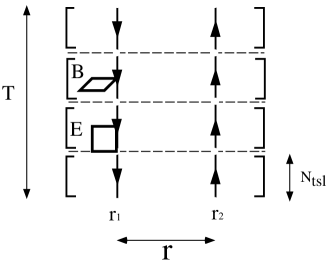
Figure 1: How to construct $\langle B_{y}(r,0)E_{z}(r,\tau)\rangle_{P^{\dagger}P}$. $[\cdots]$ denotes the sublattice average. Other correlation functions are constructed in a similar way.

We describe the procedure how to compute the field strength correlator with the PLCF background using the multi-level algorithm (here we restrict to the lowest level). The standard Wilson action is most preferable for the multi-level algorithm because its action density is locally defined. Thus we shall use this action in our simulation. Periodic boundary conditions are imposed in all directions. The essence of the multi-level algorithm is to construct the desired correlation function from the “sublattice average” of its components. In our case the corresponding parts are the two-link correlator and the field-strength-inserted two-link correlator. For a schematic understanding, see Fig. 1, which illustrates the computation of the correlation function, $\langle B_{y}E_{z}\rangle$, for $V_{1}^{\prime}$.

The sublattice is defined by dividing the lattice volume into several layers along the time direction and thus a sublattice consists of a certain number of time slices. We then take averages of the components of the correlation function at each sublattice by updating the gauge field (with a mixture of HB/OR), while the space-like links on the boundary between sublattices remain intact during the update. We repeat the sublattice update until we obtain stable signals for the components. Then, we multiply these averaged components in a desired way and complete the correlation function. This is how the correlation function is constructed from “one” configuration. We then update the whole links without specifying any layers to obtain another independent gauge configuration and start the above sublattice averaging for the next configuration.

In order to benefit from this algorithm, we need to optimize the number of time slices in each sublattice $N_{\rm tsl}$, and the number of the internal update $N_{\rm iupd}$ for sublattice averaging. They depend on the coupling $\beta$ and on the distances to be investigated. In principle, these parameters can be determined by looking at the behavior of the correlation function as a function of $N_{\rm iupd}$ for several $N_{\rm tsl}$. An empirical observation shows that $aN_{\rm tsl}=0.3-0.4$ fm is optimal in order to suppress the fluctuation of the correlation function among configurations.

3 Numerical results

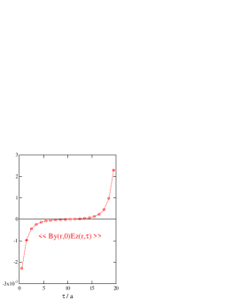
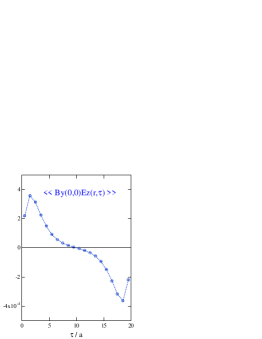
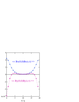
Figure 2: Correlation functions as a function of $\tau$ at $r/a=4$ on the $20^{4}$ lattice

We present the result obtained at $\beta=6.0$ ($a\approx 0.09$ fm) on the $20^{4}$ lattice, where the ranges of the measured distances between static charges are $R=2-7$. At $\beta=6.0$, we found that $N_{\rm tsl}=4$ is the optimal choice. We then chose $N_{\rm iupd}=7000$ to be able to see the signal at least up to $r/a=7$. The number of configuration is $N_{\rm conf}=76$. One Monte Carlo update consists of 1 HB/5 OR. In Fig. 2, we show the typical behavior of the correlation functions as a function of $\tau$ at $r/a=4$. We observe clean signals for the whole range of $\tau$. We also obtained similar clean data for other distances.

Once the correlation functions are obtained, our next task is to perform the integration in Eqs. (2)$-$(5) to obtain the potentials. Since the integration range of $\tau$ is limited at most to $T/2$, we need an extrapolation to extract the value corresponding to $\tau\to\infty$. This procedure is in fact the potential source of the systematic error and needs careful analysis, in particular, when the statistical errors are significantly small as shown in Fig. 2.

Currently we applied the following analysis. Since the correlation functions were reasonably smooth, we firstly performed the cubic spline interpolation of the integrand and secondly evaluated the integral analytically in the range $\tau\in[0,\tau_{\rm max}]$, where $\tau_{\rm max}=1,2,\ldots,T/2$. Then, we fitted this result with a function which has an asymptotic constant value at $\tau_{\rm max}\to\infty$, like $c+c^{\prime}\exp(-c^{\prime\prime}\tau_{\rm max})$ (exponential type) or $c/(1+(c^{\prime}/\tau_{\rm max})^{c^{\prime\prime}})$ (Hill type). The validity of the fit and the choice of the fitting function were monitored by looking at the the minimum of $\chi^{2}$ defined with the covariance matrix so as to take into account the correlation among different $\tau$’s. The errors are evaluated from the distribution of the jackknife samples of the fitting parameters.

We found that this method at least works well to extract values at $\tau_{\rm max}\to\infty$ for $V_{1}^{\prime}$, $V_{2}^{\prime}$ and $V_{3}$. The results are shown in Figs. 4 and 4 (left). For $V_{4}$, however, we found that this method needs to be modified especially at intermediate distances, because we observed a peculiar finite $\tau$ effect due to the symmetric behaviors of $\langle\!\langle B_{x}B_{x}\rangle\!\rangle$ and $\langle\!\langle B_{y}B_{y}\rangle\!\rangle$ at $\tau=T/2=10$. Thus, we just plot the integration result at $\tau_{\rm max}=9$ in Fig. 4 (right). Systematic effects of the extrapolation as well as finite volume effects will be investigated in future work.

The qualitative behaviors of these potentials are that the spin-orbit potential $V_{1}^{\prime}$ contains the long-ranged nonperturbative component ($V_{1}^{\prime}(r)$ behaves as a constant at large $r$), while $V_{3}$ and $V_{4}$ seem to be relevant at short distances. These findings are in agreement with previous works. However, the statistical errors are significantly reduced. It is interesting to find that $V_{2}^{\prime}$ is not restricted to the short range, rather it has a finite tail up to intermediate distances.

Figure 3: The spin-orbit potentials $V_{1}^{\prime}$ (left) and $V_{2}^{\prime}$ (right).

Figure 4: The spin-spin potentials $V_{3}$ (left) and $V_{4}$ (right).

4 Summary and outlook

We have measured the spin-dependent potentials in SU(3) lattice gauge theory with the Polyakov loop correlation function (PLCF) by applying the multi-level algorithm. The method presented here is promising to carry out further systematic investigations, such as the computation of the renormalization factor of the field strength operators, $Z_{B}$ and $Z_{E}$, as well as the scaling study, which are both necessary for the discussion of the fine/hyper-fine structure of the heavy quarkonium spectra.

The preliminary studies of the renormalization factors defined a la Huntley and Michael [5], but using the PLCF, show the similar values as in ref. [7]. We will report these issues in our forthcoming publication. It is also interesting to examine the Gromes relation [10], $V_{0}^{\prime}=V_{2}^{\prime}-V_{1}^{\prime}$, with high precision.

Finally we note that this method is also applicable to measuring the momentum-dependent potentials up to $O(1/m^{2})$ [11, 12] from the PLCF, since the correlation functions to be measured are quite similar to that for the spin-dependent potentials. This will help to refine the data reported in ref. [7], which is in progress.

References

- [1] E. Eichten and F. Feinberg, Spin dependent forces in heavy quark systems, Phys. Rev. Lett. 43 (1979) 1205.
- [2] Ph. de Forcrand and J.D. Stack, Spin dependent potentials in SU(3) lattice gauge theory, Phys. Rev. Lett. 55 (1985) 1254.
- [3] C. Michael, The long range spin orbit potential, Phys. Rev. Lett. 56 (1986) 1219.
- [4] M. Campostrini, K. Moriarty, and C. Rebbi, Monte carlo calculation of the spin dependent potentials for heavy quark spectroscopy, Phys. Rev. Lett. 57 (1986) 44.
- [5] A. Huntley and C. Michael, Spin-spin and spin-orbit potentials from lattice gauge theory, Nucl. Phys. B286 (1987) 211.
- [6] G.S. Bali, K. Schilling, and A. Wachter, Ab initio calculation of relativistic corrections to the static interquark potential. I: SU(2) gauge theory, Phys. Rev. D55 (1997) 5309 [hep-lat/9611025].
- [7] G.S. Bali, K. Schilling, and A. Wachter, Complete corrections to the static interquark potential from SU(3) gauge theory, Phys. Rev. D56 (1997) 2566 [hep-lat/9703019].
- [8] M. Lüscher and P. Weisz, Locality and exponential error reduction in numerical lattice gauge theory, JHEP 09 (2001) 010 [hep-lat/0108014].
- [9] Y. Koma, M. Koma, and P. Majumdar, Static potential, force, and flux-tube profile in 4D compact U(1) lattice gauge theory with the multi-level algorithm, Nucl. Phys. B692 (2004) 209 [hep-lat/0311016].
- [10] D. Gromes, Spin dependent potentials in QCD and the correct long range spin orbit term, Z. Phys. C26 (1984) 401.
- [11] A. Barchielli, E. Montaldi, and G.M. Prosperi, On a systematic derivation of the quark-antiquark potential, Nucl. Phys. B296 (1988) 625, Erratum-ibid B303 (1988) 752. .
- [12] A. Pineda and A. Vairo, The QCD potential at : Complete spin-dependent and spin-independent result, Phys. Rev. D63 (2001) 054007 [hep-ph/0009145], Erratum-ibid D64 (2001) 039902.