High Precision Fundamental Constants using Lattice Perturbation Theory

Abstract:

The HPQCD collaboration has a program for determining the fundamental constants of the Standard Model Lagrangian from lattice QCD. The most accurate method of doing this uses the $n_{f}=2+1$ improved staggered MILC ensembles with chiral fitting and multi-loop perturbative renormalisation to connect to the continuum  scheme. This program has already been very successful with the recent strong coupling constant determination at three-loops from 28 observables at three lattice spacings, and the one-loop light quark mass calculation last year. Here a preliminary result is presented for the first-ever lattice determination of the two-loop multiplicative quark mass renormalisation. The perturbative calculation involved was automated in the generation of the Feynman rules, and the generation and coding of all of the roughly 30 Feynman diagrams. The full formal framework for lattice quark mass renormalisation is given, including the cancellation of infrared divergences in intermediate diagrams. The result was checked by evaluation in three separate gauges and by two authors independently, showing the incredible flexibility and power of this perturbative methodology. Our preliminary result for the two-loop perturbative matching factor, and of systematic errors associated with higher-orders, gives  masses at a 2 GeV scale of $m_{s}=87(0)(4)(4)(0)$ MeV, and $\frac{1}{2}(m_{u}+m_{d})=3.3(0)(2)(2)(0)$ MeV, where the respective uncertainties are from lattice statistical, lattice systematic, perturbative, and electromagnetic and isospin effects. The perturbative errors are a factor of two smaller than in our previous study, and we anticipate reducing this somewhat further from additional analysis of the systematics.

PoS(LAT2005)011

1 Introduction

The strong sector of the Standard Model Lagrangian contains a number of inputs that are a priori unknown and must be determined from experiment. For these fundamental constants; the quark masses and the strong coupling constant, our knowledge is currently rather imprecise. Their determination is complicated by confinement in QCD, so the quarks and gluons cannot be observed as isolated particles. We can only determine these fundamental parameters by solving QCD for observable quantities such as hadron masses, as functions of the quark masses and the coupling (or alternatively, the lattice spacing). The High Precision QCD (HPQCD) collaboration has a program for calculating the values of these parameters using the numerical techniques of lattice QCD simulations combined with multi-loop perturbative renormalisation. Previously the masses have been determined at the one-loop level [1, 2, 3], and the strong coupling constant was determined from one observable in a two-loop calculation [4]. Recently the determination of the strong coupling was improved with three-loop perturbative matching and with input from 28 lattice observables in simulations at three different lattice spacings, resulting in an accuracy of just over 1% [5, 6]. This writeup covers progress on the determination of the light quark masses, where we push the perturbative matching calculation to two loops, that is, next-to-next-to-leading order.

Precise knowledge of quark masses constrains Beyond the Standard Model scenarios as well as providing input for phenomenological calculations of Standard Model physics. The strange quark mass, in particular, is needed for various phenomenological studies, including the important CP-violating quantity $\epsilon^{\prime}/\epsilon$ [7], where its uncertainty severely limits the theoretical precision.

Previously, shortcomings in the formulation of QCD on the lattice and limitations in computing power have meant that lattice calculations were forced to work with an unrealistic QCD vacuum that either ignored dynamical (sea) quarks or included only $u$ and $d$ quarks with masses much heavier than in nature. This condemned determinations of most phenomenologically-important quantities, including the quark masses, to rather large systematic errors (10–20%) arising from the inconsistency of comparing such unrealistic theories with the necessary experimental input. The determination presented here uses simulations with the improved staggered quark formalism that generates a much more realistic QCD vacuum with two light dynamical quarks and one strange dynamical quark. Staggered quarks are fast to simulate. They keep a remnant of chiral symmetry on the lattice, which prevents the occurrence of exceptional configurations, and which allows simulations at much smaller quark masses. The bare quark masses in the simulations were fixed using chiral perturbation theory to reliably extrapolate lattice results to the physical point [1]. Working in the region of dynamical $u/d$ quark masses below $m_{s}/2$ and down to $m_{s}/8$ gives control of chiral extrapolations and avoids the large systematic errors from dynamical quark mass and unquenching effects that afflicted previous studies using other lattice discretisations.

The dominant systematic error in the determination of the  masses in [1] came from unknown second- and higher-orders in the perturbative matching. Some progress was reported on the chiral fits at the lattice meeting [8], however that analysis is not used here; we continue to employ the bare quark masses given in [1]. Significant progress on the reduction of the systematic errors is reported here, due to our computation of the second-order perturbative matching coefficient, the first determination at this order of a “kinetic” quark mass in any lattice theory (the zero-point additive renormalisation for Wilson fermions was previously determined at two-loops in [9], and for static quarks in [10]).

The staggered quark formalism does present several challenges, which have been tamed with an aggressive program of perturbative improvement. With the naïve staggered action large discretisation errors appear, although they are formally only $\mathcal{O}(a^{2})$ or higher ($a$ is the lattice spacing). In the case of the unimproved staggered action the renormalisation of lattice operators to match to continuum quantities were also frequently large and poorly convergent in perturbation theory. This was true, for example, for the mass renormalisation that is needed here. It turns out that both problems have the same source, a particular form of discretisation error in the action, called “taste violation,” and both are ameliorated by use of the improved staggered formalism [11]. The perturbation theory then shows small renormalisations [12, 13, 14, 15] and discretisation errors are much reduced  [16, 17, 18]. Empirically, taste violation remains the most important discretisation error in the improved theory, despite being subleading to “generic” discretisation errors. The Goldstone meson masses we will discuss here are affected by this at one-loop in the chiral expansion. Staggered chiral perturbation theory (S$\chi$PT) [19, 20, 21, 22] allows us to control these effects and reduce discretisation errors significantly.

A potentially more fundamental concern about staggered fermions relates to the need to take the fourth root of the quark determinant, in order to convert the four-fold duplication of “tastes” into one quark flavor. One might imagine that the fourth root introduces nonlocalities which prevent decoupling of the ultraviolet modes of the theory in the continuum limit. However, evidence is amassing that demonstrates that the properties of the staggered theory, with the fourth root, are equivalent to a one-flavor theory, up to the expected discretisation errors. These are due to short-distance taste-changing interactions, which are mediated by high-momentum gluons [11] (the locality of the free-field staggered theory is trivial, and is made manifest in the “naive” basis used in [11]). One should not be surprised that nonlocalities do not arise, precisely because the staggered quark matrix is diagonal in the taste basis, up to those small, short-distance (and calculable) corrections. It has been demonstrated that perturbative improvement of staggered actions correlates exceedingly well with non-perturbatively measured properties of the staggered fermion matrix, providing clear support for the correctness of the fourth-root procedure. This includes the measured pattern of low-lying eigenvalues of the staggered matrix [23, 24, 25], and the measured pattern of taste-violating mass differences in the non-chiral pions [26].

The rest of this paper is organised as follows. The methodology of the calculation is discussed in the following section, including a general discussion of how to obtain the matching factor which connects the bare quark mass $m_{0}(a)$ to the  mass $m^{\msbar}(\mu)$, using the pole mass as an intermediate quantity. We also derive the two-loop anomalous dimension for the bare quark mass in the lattice-regularised theory, and give complete results for the two-loop matching coefficients. Section 3 gives preliminary results for the light quark masses, with a preliminary analysis of the systematic uncertainties, including a technique to make a rough estimate of the third-order perturbative correction. Section 4 compares our results with other recent determinations of the strange-quark mass. An appendix provides some additional information concerning the evaluation of the multi-loop diagrams, including explicit expressions for the two-loop quark mass renormalisation in terms of the 1PI self-energy, a discussion of the techniques used for generating and evaluating the necessary multi-loop integrands, and some detailed numerical results which provide an indication of the many consistency checks that we have applied to our results.

2 Structure of Calculation

The quark masses are not physically measurable, and as such are only well-defined in certain renormalisation schemes, such as the  mass $m^{\msbar}(\mu)$, evaluated at some convenient scale $\mu$. The light quark  masses are determined here by multiplying the chirally-extrapolated bare masses in lattice units, $am_{0}$, by the inverse lattice spacing $a$, and by the appropriate perturbative matching factor $Z_{m}(\mu a,m_{0}a)$, which we compute to two-loop order:

$$m^{\msbar}(\mu)=\frac{(m_{0}\,a)}{a}\;Z_{m}(\mu a,m_{0}a),$$ (1)

where the bare mass $m_{0}(a)$ is cutoff dependent. The bare masses used here were determined in an extensive chiral perturbation theory analysis of the MILC Asqtad data that was discussed in [1, 27, 28, 29]. These bare masses were previously used with the one-loop perturbation theory result for $Z_{m}$ to extract the  masses in [1]; the final result for the strange quark mass reported there was 76(0)(3)(7)(0) MeV where the respective errors are from: statistics; simulations systematics of which the most important are chiral fitting and lattice spacing; an estimate of the unknown two-loop perturbative errors and an estimate of the uncertainty due to electromagnetic and isospin contributions to the pion and kaon. That the error coming from the lattice spacing $a$ is so small is a distinguishing feature of this calculation. The lattice spacing $a$ is one of the five simulation parameters, and an important one because it sets the simulation’s mass scale. In our earlier light quark masses and $\alpha_{s}$ analyses, we set the lattice spacing by comparing a simulated $\Upsilon$ mass splitting (e.g., $\Upsilon^{\prime}-\Upsilon$) with experiment. Here we continue this practice, although the lattice spacings derived from our $\Upsilon$ splitting have been shown to agree with spacings derived from a wide variety of other physical quantities: ten in all, including the pion and kaon leptonic decay constants, the $B_{s}$ mass, and the $\Omega$ baryon mass [4, 30]. All of these different quantities agree on the lattice spacing to within 1.5–3%.

The largest error in our previous determination of the quark masses [1] was from the perturbative matching. Here that is addressed by the calculation of $Z_{m}$ at two loops. We do this in two stages, using the pole mass $M$ as a matching quantity to connect the lattice- and -regularisation schemes. We also use our previous determination of the relation between the lattice bare coupling and the renormalised coupling $\alpha_{V}(q^{*})$, defined by the static potential, to reorganise both sides of the matching equation into series in terms of $\alpha_{V}(q^{*})$ at an appropriately determined scale.

We begin by recalling the relation between the  mass and the pole mass $M$, which is known through three loops [31, 32, 33, 34, 35]. We require it to second order, a result that was first obtained in [32] (expressions for the relation at arbitrary $\mu$ are conveniently given in [34])

$$m^{\msbar}(\mu)=M\left[1+z_{1}\left(\frac{\mu}{M}\right)\frac{\alpha_{\msbar}(\mu)}{\pi}+z_{2}\left(\frac{\mu}{M}\right)\frac{\alpha^{2}_{\msbar}(\mu)}{\pi^{2}}+\ldots\right],$$ (2)

where the one- and two-loop coefficient functions $z_{1}(\mu/M)$ and $z_{2}(\mu/M)$ are reduced to a set of terms with different colour structures [in the following $C_{F}=(N_{c}^{2}-1)/(2N_{c})$, $C_{A}=N_{c}$, and $T=1/2$]

$$z_{1} =C_{F}z_{F}$$ (3)

$$z_{2} =C_{F}^{2}z_{FF}+C_{F}C_{A}z_{FA}+C_{F}Tn_{\ell}z_{FL}+C_{F}Tz_{FH},$$ (4)

and where the contribution $z_{FH}$ from an internal quark loop with the same flavor as the valence quark is split off from the contribution $z_{FL}$ of $n_{\ell}$ internal quark loops with different flavor (these are taken here to be degenerate in mass, though this is easily generalised). The total number of flavors is $n_{f}=n_{\ell}+1$. The individual functions are given by

$$z_{F} =-1-{\textstyle{\frac{3}{4}}}\ell_{\mu M},$$ (5)

$$z_{FF} ={\textstyle{\frac{7}{128}}}-{\textstyle{\frac{15}{8}}}\zeta_{2}-{\textstyle{\frac{3}{4}}}\zeta_{3}+3\zeta_{2}\log 2+{\textstyle{\frac{21}{32}}}\ell_{\mu M}+{\textstyle{\frac{9}{32}}}\ell_{\mu M}^{\,2},$$ (6)

$$z_{FA} =-{\textstyle{\frac{1111}{384}}}+{\textstyle{\frac{1}{2}}}\zeta_{2}+{\textstyle{\frac{3}{8}}}\zeta_{3}-{\textstyle{\frac{3}{2}}}\zeta_{2}\log 2-{\textstyle{\frac{185}{96}}}\ell_{\mu M}-{\textstyle{\frac{11}{32}}}\ell_{\mu M}^{\,2},$$ (7)

$$z_{FL} ={\textstyle{\frac{71}{96}}}+{\textstyle{\frac{1}{2}}}\zeta_{2}-2\Delta(r_{\rm sea})+{\textstyle{\frac{13}{24}}}\ell_{\mu M}+{\textstyle{\frac{1}{8}}}\ell_{\mu M}^{\,2},$$ (8)

$$z_{FH} ={\textstyle{\frac{71}{96}}}+{\textstyle{\frac{1}{2}}}\zeta_{2}-2\Delta(1)+{\textstyle{\frac{13}{24}}}\ell_{\mu M}+{\textstyle{\frac{1}{8}}}\ell_{\mu M}^{\,2},$$ (9)

where $\ell_{\mu M}\equiv\log(\mu^{2}/M^{2})$, and where the function $\Delta(r)$ gives the dependence of the renormalisation factors $z_{FL}$ and $z_{FH}$ on the quark mass in an internal fermion loop (sea and valence, respectively), with $r_{\rm sea}=m_{\rm sea}/m_{\rm valence}$. An exact integral expression for $\Delta(r)$ can be found in [32] and it is plotted in the appendix.

Next we outline the computation of the relation between the pole mass $M$ and the bare quark mass $m_{0}(a)$ in the lattice-regularised theory, which has the form

$$M=m_{0}\left[1+\alpha_{L}\left(A_{11}\log m_{0}a+A_{10}\right)+\alpha_{L}^{2}\left(A_{22}\log^{2}m_{0}a+A_{21}\log m_{0}a+A_{20}\right)+\ldots\right].$$ (10)

The coefficients of the logarithms are determined by the two-loop anomalous dimension in $m_{0}(a)$, which in turn can be determined from the known anomalous dimension of the $\msbar$ mass, as described below. We have previously computed the one-loop matching factor, with the result [1, 12] $A_{10}\approx 0.5432$ (neglecting corrections of $O((am_{0})^{2})$). What is new in this paper is the determination of the two-loop term $A_{20}$.

As with the two-loop continuum matching factor in (2), $A_{20}$ depends on the number of quark flavors in the sea, and on the ratios of the sea quark masses $m_{\rm sea}$ to the valence quark mass $m_{\rm valence}$. However, as we demonstrate explicitly in the appendix, the mass dependence in $A_{20}$ cancels precisely in the matching to the continuum relation (2) for $m_{\text{sea}}/m_{\text{valence}}$ in the range necessary. This follows from the fact that, in the limit where the energy scales are large, the net renormalisation factor connecting $m_{0}(a)$ to $m^{\msbar}(\mu)$ probes internal loops at scales large compared to the internal quark masses; hence the dependence on quark masses of the intermediate renormalisation factors connecting to the pole mass $M$ are infrared effects that are identical in the lattice- and -regularised theories.

Before we give our results for $A_{20}$, and the final matching factor $Z_{m}$ in (1), we consider how to determine the coefficients of the logarithmic terms in (10). The pole mass is an RD invariant (equivalently does not depend on $a$) so taking logs and differentiating with respect to $\log a$, and neglecting any scale dependence in the coefficients $A_{nm}$ (which would arise as discretisation errors that go as powers of $m_{0}a\lesssim 0.05$, which are negligible for our purposes), one has

$$0=\frac{d\log m_{0}}{d\log a}+\frac{d}{d\log a}\Biggl{\{}\Bigl{[}\cdots\Bigr{]}-\frac{1}{2}\Bigl{[}\cdots\Bigr{]}^{2}\Biggr{\}},$$ (11)

where the square bracket is from (10), and the first term above can be identified with the anomalous dimension equation:

$$\frac{d\log m_{0}}{d\log a}\equiv\gamma_{0}\,\alpha_{L}(a)+\gamma_{1}^{L}\,\alpha_{L}^{2}(a)+\mathcal{O}(\alpha_{L}^{3})$$ (12)

The $L$’s indicate the lattice-regularisation scheme. The sign comes from differentiating with respect to the logarithm of the lattice scale $a^{-1}$ (momentum units), instead of $\mu$. Only the leading term in the anomalous dimension is scheme independent, $\gamma_{0}=3C_{F}/(2\pi)$. Comparison of the two preceding equations leads to the identification

$$A_{11}=-\gamma_{0},\qquad A_{22}=\frac{1}{2}A_{11}^{2}-A_{11}\frac{\beta_{0}}{4\pi},\qquad A_{21}=-\gamma_{1}^{L}+A_{11}^{2}-A_{10}\left(\frac{\beta_{0}}{2\pi}-A_{11}\right),$$ (13)

where the $\beta$-function arises from an implicit derivative of the bare lattice coupling in (11) ($\beta_{0}=11-\frac{2}{3}n_{f}$). It remains to determine $\gamma_{1}^{L}$. This can be found from the known  anomalous dimension,

$$-\frac{d\log m_{\msbar}}{d\log\mu} \equiv\gamma_{0}\alpha_{\msbar}(\mu)+\gamma_{1}^{\msbar}\alpha_{\msbar}^{2}(\mu)+\mathcal{O}(\alpha^{3}),\qquad\gamma_{1}^{\msbar}=\frac{101}{12\pi^{2}}-\frac{10}{36\pi^{2}}n_{f},$$ (14)

making the substitution $\mu=a^{-1}$, and using the relations $m_{\msbar}(a^{-1})=m_{0}(1+C_{m}\alpha)$, and $\alpha_{\msbar}(a^{-1})=\alpha_{L}(1+C_{\alpha}\alpha_{L})$. By comparison to (12) we obtain

$$\gamma_{1}^{L} =\gamma_{1}^{\msbar}+C_{\alpha}\gamma_{0}-C_{m}\frac{\beta_{0}}{2\pi}.$$ (15)

The one-loop renormalisation constants $C_{m}=Z_{m}^{(2)}(\mu=1/a)=0.1188$ and $C_{\alpha}=4.753-0.3316n_{f}$ for the improved gluon and staggered quark actions have been previously calculated [1, 12, 5, 6].

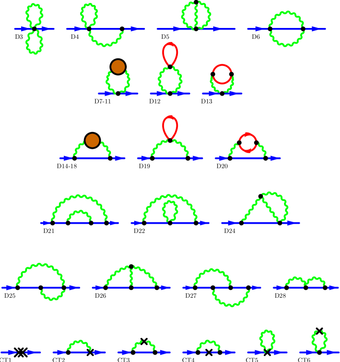
Figure 1: The two-loop diagrams that contribute to the two-loop mass renormalisation. The numbering is consistent with [9]. Blue lines are valence quarks (on-shell externally), green are gluons and red are sea quarks. The large brown vertices are stand-ins for the five one-loop gluon propagator diagrams (gluon and ghost bubbles and tadpoles and the measure term). We evaluate all five simultaneously with an internal subtraction. The crosses represent interaction vertices generated by perturbative expansion of tadpole and other renormalisation factors in the gluon and quark actions.

Knowing the logarithmic terms due to the lattice anomalous dimension provides a useful cross-check on our evaluation of the two-loop renormalisation factor (10). We compute the two-loop lattice diagrams as a function of $m_{0}a$, and subtract the known logarithms, in order to isolate the remaining term $A_{20}$, which must be finite as $m_{0}a\to 0$. Additional checks are provided for diagrams which have a leading $\log^{2}(am_{0})$ term, which arises from the infrared limit of both the outer and inner loop integrals, and which is therefore an infrared quantity; the coefficients of the double logarithms in the individual diagrams are available in Feynman gauge from the original  calculation of Tarrach [31], and we have verified that these are reproduced in our lattice calculation.

The necessary two-loop diagrams are shown in figure 1. Further details on our evaluation of these diagram are given in the appendix. We can easily evaluate them for various gluon and quark actions, using our automated methods for generating the lattice Feynman rules. In this paper we give results for the Symanzik improved gluon with improved staggered quarks (Asqtad) and SU(3). Our result for the matching term $A_{20}$ is, in the limit of vanishing sea quark mass,

$$A_{20}=6.09-0.15n_{\ell}-0.03,$$ (16)

where the last term corresponds to an internal quark loop containing one (massive) valence quark flavor. The uncertainties arise from a numerical evaluation of the two-loop integrals.

When the lattice renormalisation factor (10) connecting the bare mass to the pole mass is combined with the equivalent continuum expression (2) for the connection to the  mass, the logs of $m_{0}$ drop out, as expected, since these are infrared effects that are identical in the intermediate lattice and continuum matchings. We also reorganise the couplings to the $\alpha_{V}$ scheme at some scale $q^{*}$, where $q^{*}a$ is a function of $\mu a$ that is determined according to the BLM scheme [39]. This leaves an expression with logarithms only of $\mu a$ and $q^{*}a$. The final expression for the perturbative matching factor is then:

$$Z_{m}(\mu a,m_{0}a)=1+Z_{m}^{(2)}(\mu a)\alpha_{V}\left(q^{*}(\mu a)\right)+Z^{(4)}_{m}(\mu a)\alpha_{V}^{2}+\mathcal{O}((m_{0}a)^{4},(m_{0}a)^{2}\alpha^{2},\alpha^{3}),$$ (17)

where $Z_{m}^{(2)}(\mu a)=0.1188(1)-2/\pi\log(\mu a)+\mathcal{O}(m_{0}a)^{2}$ was derived previously, [1], and the new information presented here is the expression for $Z_{m}^{(4)}$

$$Z_{m}^{(4)}(\mu a)=Z_{2}\log^{2}(\mu a)+Z_{1}\log(\mu a)+Z_{0},$$ (18)

where the latter coefficients depend on logarithms of $q^{*}a$

$$Z_{2} =0.76-0.034n_{f}$$ (19)

$$Z_{1} =-0.40-0.028n_{f}+(-1.12+0.0675n_{f})\ln q^{*}a$$ (20)

$$Z_{0} =2.09-0.014n_{f}+(0.21-0.013n_{f})\ln q^{*}a.$$ (21)

We have computed the optimal choice for $q^{*}a$ in the BLM scheme, as a function of $\mu a$, using an exact evaluation of the average momentum scales in the continuum self-energy diagrams, according to [39] (this is an improvement over the inexact calculation in [1]), and a numerical evaluation of the average scales in the lattice self-energy (unchanged). A typical value for the matching scale is $q^{*}a=1.88$ at $\mu a=1$.

3 Results

The bare lattice masses for the strange and up/down quarks, on the MILC “coarse” and “fine” lattices, are given in [1]. For the strange quark, these are $am_{0s}=0.0390(1)(20)/u_{0c}$, and $am_{0s}=0.0272(1)(12)/u_{0f}$, on the coarse and fine lattices respectively, where $u_{0c}=0.85488$ and $u_{0f}=0.86774$ are tadpole normalisation factors. The uncertainties are lattice statistical and systematic errors, respectively, the latter due mainly to chiral extrapolation/interpolation. The lattice spacings can be found in [5], $a^{-1}_{\rm coarse}=1.596(30)$ GeV, and $a^{-1}_{\rm fine}=2.258(32)$ GeV.

Following conventional practice, we quote the light quark  masses at the scale $\mu=2$ GeV, taking three active flavors of quarks ($n_{f}=3$). This results in two-loop coefficients in (17) of $Z_{m}^{(4)}|_{\rm coarse}=1.939(4)$, and $Z_{m}^{(4)}|_{\rm fine}=2.270(4)$. Finally, we require the couplings at the relevant scales, and for this purpose we use the recently determined value $\alpha_{V}^{(n_{f}=3)}(7.5~{}\mbox{GeV})=0.2082(40)$ [5]. We find $\alpha_{V}(q^{*}_{\rm coarse})=0.2925(92)$ and $\alpha_{V}(q^{*}_{\rm fine})=0.2713(76)$.

Putting all of this together, we obtain the following preliminary values for the  strange-quark mass, using the coarse and fine lattices as input

$$m^{\msbar}_{s}(2~{}\mbox{GeV})=83(5)~{}\mbox{MeV\ [coarse]},\quad m^{\msbar}_{s}(2~{}\mbox{GeV})=85(4)~{}\mbox{MeV\ [fine]},$$ (22)

where the errors here are just from the simulation systematics.

Following [1], we consider continuum extrapolations of the central values in (22) based on the form of the expected leading discretisation errors, which are of $O(\alpha_{V}a^{2})$, and compare with a extrapolation in $\alpha_{V}^{2}a^{2}$. These two forms yield almost identical extrapolations, to a central value of 87 MeV, with an error that is folded into the quoted lattice systematic errors above. We are currently considering refinements to our estimates of the continuum extrapolation and the incorporation of third order perturbative errors. For this preliminary result we quote as our continuum extrapolation

$$m^{\msbar}_{s}(2~{}\mbox{GeV})=87(0)(4)(4)(0)~{}\mbox{MeV}$$ (23)

where, following [1], the respective errors are statistical, lattice systematic, perturbative, and electromagnetic. We have assigned a relative error from the estimated third-order perturbative matching of roughly $\pm 2\alpha^{3}_{V}(q^{*})\approx 5\%$, down from the 10% perturbation theory error in the one-loop determination in [1]. We anticipate to reduce somewhat the perturbation theory error with a more careful study of the systematics of the $\mu$ dependence.

Our result for the ratio of strange to up/down quark masses is unchanged at 27.4(1)(4)(0)(1) from [1], since the renormalisation factor is mass-independent, as we have verified above explicitly through two-loops. Using the value $m_{u}/m_{d}=0.43(0)(8)(1)(0)$ from [28] this gives:

$$m^{\msbar}_{u}(2~{}\mbox{GeV})=1.9(0)(1)(1)(2)~{}\mbox{MeV}$$

$$m^{\msbar}_{d}(2~{}\mbox{GeV})=4.4(0)(2)(2)(2)~{}\mbox{MeV}$$

4 Discussion and Conclusions

Perturbation theory has once again shown itself to be an essential tool in high precision phenomenological calculations from the lattice. The two-loop lattice diagrams were conquered with a combination of algebraic and numerical techniques in this first-ever determination of the multiplicative two-loop pole mass on the lattice. When combined with the known continuum matching from the pole mass to the  mass, a very accurate determination of the light quark masses was possible. The results presented here have a number of distinguishing features: two-loop perturbation theory, $n_{f}=2+1$ simulations with two degenerate light quarks and a heavier strange quark, very small light quark masses from $m_{s}/8$ to $m_{s}/2$ which enabled a partially quenched chiral fit with many terms to thousands of configurations, and extremely accurate determinations of the lattice spacings, which are equal within the errors when set from any of 10 different quantities, ranging from the very lightest states all the way up to heavy mesons and baryons [4, 30].

Most notable amongst our results is our new value for strange quark mass $m^{\msbar}_{s}(2~{}\mbox{GeV})=87(0)(4)(4)(0)~{}\mbox{MeV}$, where the respective errors are lattice statistical, lattice systematic (mostly due to the chiral extrapolation/interpolation), perturbative, and due to electromagnetic effects. The two-loop matching has increased the central value with respect to the previous determination in [1] by about two standard deviations, based on the previous estimate of the perturbation theory uncertainty (which was $\pm 7$ MeV). We believe the present estimate of the perturbative uncertainty of $\pm 4$ MeV can be reduced somewhat by estimating the third-order perturbative correction, along the lines that we have already explored, in a preliminary way, here.

The strange quark mass determination has historically generated some controversy, with somewhat different values being obtained from different approaches. An obvious advantage of our result is that it has been obtained with the correct description of the sea, that is, with $n_{f}=2+1$ flavors of dynamical quarks. There is only one other result with the correct number of flavors in the sea, which is due to the CP-PACS and JLQCD collaborations, who reported a value at this conference of $m^{\msbar}_{s}(2~{}\mbox{GeV})=87(6)$ MeV [40], although the error was not very well quantified, and does not appear to include an estimate of corrections due to two-loop and higher-orders in the perturbative matching.

It appears the the strange-quark mass extracted from simulations with only $n_{f}=2$ flavors of sea quarks are systematically higher than the estimates with the correct $n_{f}$ (noting that the two-flavor determinations were also done with nonperturbative definitions of the quark mass), although the other systematic errors are too large to allow for a definitive assessment. The two-flavor determination from the QCDSF-UKQCD collaboration, is $m^{\msbar}_{s}(2~{}\mbox{GeV})=100-130$ MeV [41], the ALPHA collaboration value is $97(22)$ MeV [42], and the Rome value is $101(8)(^{+25}_{-9}$) MeV [43].

The next major evolution in our lattice determination of the light quark masses will come from using a third lattice spacing, the “super-fine” configurations already partially implemented by MILC, and planned by UKQCD. This will hopefully reduce the size of the chiral and systematic errors due to taste-breaking, and vastly improve the quality of the continuum extrapolation. The HPQCD collaboration plans to continue its accurate determinations of the fundamental constants by generalising this calculation in the first instance to heavy quark masses to complete the strong sector of the Standard Model Lagrangian with two-loop calculations of all the quark masses with the already finished three-loop strong coupling constant. Further generalisation by insertion of appropriate operators will give the two-loop vector and axial-vector renormalisations, necessary for improving the accuracy of the decay constants $f_{B}$, $f_{D}$ etc and associated form-factors. Eventually HPQCD plans therefore to have two-loop accurate determinations of many of the CKM matrix elements in the next few years.

Appendix A Perturbative Structure

We present some details of the lattice size of the pole mass renormalisation factor, (10). We define the full lattice quark propagator to be:

$$G(p,m_{0})^{-1}=i\widehat{p}\hbox to0.0pt{\hss$/$}+m_{0}+\Sigma_{\rm tot}(p),$$ (24)

where $\Sigma_{\rm tot}$ is minus the usual 1PI truncated two-point function. The lattice dispersion relation implied by $\hat{p}$ will be kept as a general function of the lattice momentum $p$; for unimproved staggered quarks, for instance, $\hat{p}_{\mu}=\sin(p_{\mu})$. Make the spinor decomposition:

$$\Sigma_{\rm tot}(p)=\Sigma_{1}(p)+(i\widehat{p}\hbox to0.0pt{\hss$/$}+m_{0})\,\Sigma_{2}(p),$$ (25)

where both $\Sigma_{1}$ and $\Sigma_{2}$ are implicitly functions of $m_{0}$, and both are Dirac scalars. Note that $\Sigma_{2}$ is only part of the wavefunction renormalisation. The pole mass is defined by the all-orders on-shell condition, corresponding to the location of the pole in the propagator. At tree-level this is “$-i\widehat{p}\hbox to0.0pt{\hss$/$}=m_{0}$” (a very common but abusive notation). As is conventional, we work at zero external three momentum, $p=(p_{t},\vec{0})$, and use the positive energy spinor projector (Euclidean), $(1+\gamma_{t})/4$. Then it is convenient to rearrange (24) and (25) to get

$$P(p_{t})\equiv-i\widehat{p}_{t}=m_{0}+\frac{\Sigma_{1}(p)}{1+\Sigma_{2}(p)}$$ (26)

This relation can also be applied to theories with an additive mass renormalisation, such as Wilson quarks, by absorbing the momentum dependence of the additive mass into $P(p_{t})$.

We recursively solve (26) for the on-shell pole mass $M$, defined by the renormalised energy at zero three-momentum

$$p_{t}=iM,\qquad\text{where}\;M=M^{(0)}+g_{0}^{2}M^{(2)}+g_{0}^{4}M^{(4)},$$ (27)

is the perturbative expansion, with a corresponding series for other quantities (including e.g. $p_{t}^{(0)}=iM^{(0)}$ and $P(iM^{(0)})=m_{0}$).

We first consider the expansion of (26) through one-loop, which reads

$$P(iM^{(0)}+ig_{0}^{2}M^{(2)})=m_{0}+g_{0}^{2}\Sigma_{1}^{(2)}(p^{(0)}).$$ (28)

Hence

$$M^{(2)} =Z_{\Psi}^{(0)}\,\Sigma_{1}^{(2)}(p^{(0)}),\quad\text{where}\;{Z_{\Psi}^{(0)}}^{-1}=\left.\frac{dP(ix)}{dx}\right|_{x=M^{(0)}},$$ (29)

is the tree-level wave function residue (e.g. $Z_{\Psi}^{(0)}=1/\cosh(M^{(0)})$ for unimproved staggered quarks).

To find the location of the pole at two-loops requires solving (24) self-consistently

$$P(iM^{(0)}+ig_{0}^{2}M^{(2)}+ig_{0}^{4}M^{(4)}) =m_{0}+g_{0}^{2}m^{(2)}+g_{0}^{4}m^{(4)},$$

where the right-hand side above represents a self-consistent expansion of the right-hand side of (26). Part of the $O(g_{0}^{4})$ term arises from the one-loop piece of $\operatorname{\Sigma}_{1}$ when it is evaluated at the one-loop-corrected on-shell energy $p_{t}$, determined by (27) and (29). By Taylor expansion:

$$\Sigma_{1}^{(2)}(p_{t})=\Sigma_{1}^{(2)}(iM^{(0)})+ig_{0}^{2}\,M^{(2)}\left.\frac{\partial\Sigma_{1}^{(2)}(p_{t})}{\partial p_{t}}\right|_{p_{t}=iM^{(0)}}+\mathcal{O}(g_{0}^{4}).$$ (30)

The result for the two-loop contribution to the pole mass is therefore

$$M^{(4)} =Z_{\psi}^{(0)}\left(m^{(4)}-\frac{1}{2}(M^{(2)})^{2}{\left.\frac{d^{2}P(ix)}{dx^{2}}\right|_{x=M^{(0)}}}\right)$$ (31)

(the second-term above is a correction of $O((am_{0})^{4})$ for Asqtad), and

$$m^{(4)}=\Sigma_{1}^{(4)}(iM^{(0)})+\Sigma_{1}^{(2)}(iM^{(0)})\,Z_{\psi}^{(0)}\left\{\operatorname{Tr}\left[\frac{1+\gamma_{t}}{4}\frac{\partial\Sigma_{\rm tot}^{(2)}(p_{t})}{\partial p_{t}}\right]_{p_{t}=iM^{(0)}}\right\},$$ (32)

where the identity

$$Z_{\psi}^{(0)}\operatorname{Tr}\left[\frac{1+\gamma_{t}}{4}\frac{\partial\Sigma_{\rm tot}^{(2)}(p_{t})}{\partial p_{t}}\right]_{p_{t}=iM^{(0)}}=-\Sigma_{2}^{(2)}(iM^{(0)})+\left.i\frac{\partial\Sigma_{1}^{(2)}(p_{t})}{\partial p_{t}}\right|_{p_{t}=iM^{(0)}}$$ (33)

was used. In the continuum, $Z_{\psi}^{(0)}=1$ and (33) is the complete one-loop expression for the wave function renormalisation there. On the lattice, which has a tree level wavefunction renormalisation the result has some additional terms:

$$Z_{\Psi}^{-1}={Z_{\Psi}^{(0)}}^{-1}+g_{0}^{2}\Biggl{\{} i\operatorname{Tr}\left[\frac{1+\gamma_{t}}{4}\frac{\partial\Sigma^{(2)}_{\text{tot}}(p)}{\partial p_{t}}\right]_{p=p^{(0)}}+M^{(2)}\left.\frac{d^{2}P(ix)}{dx^{2}}\right|_{p=p^{(0)}}\Biggr{\}}.$$

Unfortunately (33) is IR divergent for both lattice and continuum. This infrared divergence precisely cancels against an IR divergence in the two-loop nested-rainbow diagrams (D21, D22 and CT4 in figure 1). This parallels the cancellation of an infrared divergence in the continuum two-loop diagram, D21, , which is likewise rendered finite by the iteration of the the one-loop self-energy, which generates a “counterterm” given by the one-loop mass shift times the one-loop wave function residue, analogous to the terms in (32).

In this connection, we note that the continuum pole mass was shown to be infrared finite at two-loops by Tarrach [31]; an all-orders proof of the finiteness of the on-shell self-energy has only recently been established, by Kronfeld [36].

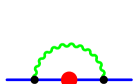
$\!\!+\,iZ_{\Psi}^{(0)}\Bigl{\{}$ $\Bigr{\}}\frac{\partial}{\partial p_{t}}\!\Bigl{\{}$ ​$\!\Bigr{\}}=$ IR finite,

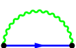
where $\!\!\equiv$ , and

Figure 2: Schematic representation of an IR subtraction, where appropriate traces of the self-energy with an energy-projector are implicit in this schematic representation.

On the lattice, the infrared cancellation in (32) has a schematic representation in diagrammatic form, as shown in figure 2. We numerically evaluate the integral for the two-loop diagram on the left in figure 2 with a subtraction, in its integrand, of the product of the independent integrands for the one-loop self-energy, and its derivative. This grouping, as indicated in figure 2, is IR finite, and does not require any infrared regulator. We obtain a powerful check of this result by noting that this combination generates a leading logarithmic contribution to the anomalous dimension of the mass which goes like $\log^{2}(a^{2}m_{0}^{2})$, and whose coefficient is identical to that of the infrared-subtracted combination in the continuum, which can be found in Feynman gauge from the  results in [31].

All the diagrams for the two-loop self-energy, figure 1, were generated and evaluated independently by two of us. The Feynman rules for the highly-improved actions are exceedingly complicated, and were generated automatically using computer algebra-based codes [14]. Moreover, one of us has produced an algorithm which automatically generates the Feynman diagrams themselves [37]. The two-loop integrals were evaluated numerically, using the adaptive Monte-Carlo sampling of method of VEGAS [38]. Practically, when performing the subtractions of figure 2 the integrals are much more convergent with a (4D) spherical transform and a further $k_{\text{new}}=\log|k|$ transformation. The effect of the associated Jacobian’s is to regulate the IR with $k^{4}$ and a spherical cut-off at small $|k|$. We found that $e^{-10}$ and smaller were sufficient to show the integrals independent of this cut-off. Almost all diagrams benefited from using the spherical transform, though some of the other “continuum” like diagrams are better behaved with the “log-spherical” transform for very large numbers of integrand evaluations. We have checked that varying the cut-off makes no difference to the result. A powerful additional cross-check was provided by an explicit verification that our results are gauge independent, which we established numerically for two different bare-quark masses in three covariant gauges: Feynman, Landau and Yennie.

We show results for the two-loop part of the pole mass, (10), coming from diagrams without fermion loops, in figure 3. As described in Sect. 2, we can test our calculation by subtracting the known logarithms in $m_{0}a$, in order to expose the remaining factor $A_{20}$, which must be finite in the limit $m_{0}a\to 0$. Figure 3 shows results for the gluonic part of $A_{20}$ over a wide range of bare masses, which clearly shows the expected limiting behaviour.

\psfrag{ylabel}[cc][1.5]{\large$A_{20}|_{n_{f}=0}$ in $\alpha_{L}^{2}$}\psfrag{TOT Imp}[cc][1.5]{\large Asqtad multiplicative mass renormalisation at two-loops}\psfrag{Quark Mass}[cc][1.5]{\large Quark Mass $(m_{0}a)$}\includegraphics[angle={-90},width=361.34999pt,clip]{Results.ps}

Figure 3: The total of the gluonic part of the two-loop contribution to the pole mass on the lattice with the Asqtad action, evaluated independently by two of the authors, in units of $\alpha_{L}^{2}$, for varying quark mass $(m_{0}a)$. The data is shown after subtracting the known logarithms: $A_{22}\log^{2}m_{0}a+A_{21}\log m_{0}a$, and should therefore be the constant, $A_{20}$, with no mass dependence. The absence of observed lattice artifacts of the form $(m_{0}a)^{n}\log^{l}m_{0}a$, $l\leq 2$ justifies our assumption in the derivation that for small masses the lattice is a mass-independent renormalisation scheme.

A further stringent check of our evaluation of the diagrams with internal fermion loops (diagrams 12, 13, 19 and 20 in figure 1) is achieved by computing over a range of sea quark masses. As described in Sect. 3, the mass dependence in the intermediate renormalisation from the bare mass to the pole mass $M$ should cancel against the renormalisation from $M$ to the  mass. We define

$$A_{20}(r_{\rm sea})\equiv A_{20}(0)+\frac{4}{3\pi^{2}}\Delta_{\rm lattice}(r_{\rm sea}),\quad r_{\rm sea}=\frac{m_{\rm sea}}{m_{\rm valence}},$$ (34)

and compare with the analogous continuum function $\Delta(r_{\rm sea})$. We plot our results in figure 4, over a very wide range in $r_{\rm sea}$, which shows the expected cancellation.

Figure 4: Comparison of the sea loop-quark mass dependence of pole mass renormalisation matching factors, on the lattice-side of the matching, and on the continuum side. The difference between the continuum squares and lattice crosses (calculated at $am_{\text{valence}}=0.001$), is smaller than the errors. The variable $r=m_{\rm sea}/m_{\rm valence}$. The solid lines show limiting forms of the dilogarithmic but analytic continuum function.

References

- [1] C. Aubin et al. (HPQCD, MILC, UKQCD), Phys. Rev. D. 70 031504 (2004) [hep-lat/0405022].
- [2] M. Nobes and H. Trottier, [hep-lat/0509128].
- [3] A. Gray, I. Allison, C. T. H. Davies, E. Gulez, G. P. Lepage, J. Shigemitsu and M. Wingate, [hep-lat/0507013].
- [4] C. T. H. Davies et al. (Fermilab, HPQCD, MILC, UKQCD), Phys. Rev. Lett. 92 022001 (2004) [hep-lat/0309088].
- [5] Q. Mason et al. (HPQCD), Phys. Rev. Lett. 95 052002 (2005) [hep-lat/0503005].
- [6] Q. Mason and H. D. Trottier, in preparation.
- [7] A. J. Buras, M. Jamin and M. E. Lautenbacher, Phys. Lett. B389, 749 (1996) [hep-ph/9608365].
- [8] C. Bernard et al., [MILC Collaboration], [hep-lat/0509137].
- [9] E. Follana and H. Panagopoulos, Phys. Rev. D 63 017501 (2000) [hep-lat/0006001].
- [10] G. Martinelli and C. T. Sachrajda, Nucl. Phys. B 559, 429 (1999) [hep-lat/9812001].
- [11] G. P. Lepage, Phys. Rev. D 59, 074502 (1999) [hep-lat/9809157].
- [12] J. Hein, Q. Mason, G. P. Lepage and H. Trottier, Nucl. Phys. Proc. Suppl. 106, 236 (2002) [hep-lat/0110045]. M. A. Nobes, H. D. Trottier, G. P. Lepage and Q. Mason, ibid., 838 [hep-lat/0110051].
- [13] W. J. Lee and S. R. Sharpe, Phys. Rev. D 66, 114501 (2002) [hep-lat/0208018].
- [14] H. D. Trottier, Nucl. Phys. Proc. Suppl. 129, 142 (2004) [hep-lat/0310044].
- [15] Q. Mason et al. (HPQCD), Nucl. Phys. Proc. Suppl. 119, 446 (2003) [hep-lat/0209152].
- [16] T. Blum et al., Phys. Rev. D 55, 1133 (1997) [hep-lat/9609036].
- [17] C. W. Bernard et al. [MILC Collaboration], Phys. Rev. D 58, 014503 (1998) [hep-lat/9712010].
- [18] K. Orginos and D. Toussaint [MILC collaboration], Phys. Rev. D 59, 014501 (1999) [hep-lat/9805009].
- [19] W. J. Lee and S. R. Sharpe, Phys. Rev. D 60, 114503 (1999) [hep-lat/9905023].
- [20] C. Bernard [MILC Collaboration], Phys. Rev. D 65, 054031 (2002) [hep-lat/0111051].
- [21] C. Aubin and C. Bernard, Phys. Rev. D 68, 034014 (2003) [hep-lat/0304014].
- [22] C. Aubin et al. [MILC Collaboration], Nucl. Phys. Proc. Suppl. 129, 227 (2004) [hep-lat/0309088].
- [23] E. Follana, A. Hart and C. T. H. Davies, Phys. Rev. Lett. 93, 241601 (2004) [hep-lat/0406010].
- [24] K. Y. Wong and R. M. Woloshyn, Phys. Rev. D 71, 094508 (2005) [hep-lat/0412001].
- [25] S. Durr, C. Hoelbling and U. Wenger, Phys. Rev. D 70, 094502 (2004) [hep-lat/0406027].
- [26] E. Follana, C. Davies, A. Hart, P. Lepage, Q. Mason and H. Trottier [HPQCD Collaboration], Nucl. Phys. Proc. Suppl. 129& 130, 384 (2004) [hep-lat/0406021].
- [27] C. Aubin et al. [MILC Collaboration], Phys. Rev. D 70, 094505 (2004) [hep-lat/0402030].
- [28] C. Aubin et al. [MILC Collaboration], Phys. Rev. D 70, 114501 (2004) [hep-lat/0407028].
- [29] S. A. Gottlieb, Nucl. Phys. Proc. Suppl. 128, 72 (2004) [hep-lat/0310041].
- [30] D. Toussaint and C. T. H. Davies, Nucl. Phys. Proc. Suppl. 140, 234 (2005) [hep-lat/0409129].
- [31] R. Tarrach, Nucl. Phys. B 183, 384 (1981).
- [32] N. Gray, D. J. Broadhurst, W. Grafe and K. Schilcher, Z. Phys. C 48, 673 (1990).
- [33] D. J. Broadhurst, N. Gray and K. Schilcher, Z. Phys. C 52, 111 (1991).
- [34] K. G. Chetyrkin and M. Steinhauser, Nucl. Phys. B 573, 617 (2000) [hep-ph/9911434].
- [35] K. Melnikov and T. v. Ritbergen, Phys. Lett. B 482 (2000) 99 [hep-ph/9912391].
- [36] A. S. Kronfeld, Phys. Rev. D 58, 051501 (1998) [hep-ph/9805215].
- [37] Q. J. Mason, Ph.D. thesis, Cornell University (2004).
- [38] G. P. Lepage, J. Comput. Phys. 27 192 (1978).
- [39] S. J. Brodsky, G. P. Lepage and P. B. Mackenzie, Phys. Rev. D 28, 228 (1983). K. Hornbostel, G. P. Lepage and C. Morningstar, Phys. Rev. D 67, 034023 (2003) [hep-ph/0208224].
- [40] T. Ishikawa et al. [CP-PACS and JLQCD collaborations], [hep-lat/0509142].
- [41] M. Gockeler et al. [QCDSF-UKQCD collaboration], [hep-lat/0509159].
- [42] M. Della Morte et al. [ALPHA collaboration], [hep-lat/0509073].
- [43] D. Becirevic et al., [hep-lat/0509091].