Fluctuations, strangeness and quasi-quarks
in heavy-ion collisions from lattice QCD

Abstract

We report measurements of diagonal susceptibilities for the baryon number, $\chi_{B}$, electrical charge, $\chi_{Q}$, third component of isospin, $\chi_{I}$, strangeness, $\chi_{S}$, and hypercharge, $\chi_{Y}$, as well as the off-diagonal $\chi_{BQ}$, $\chi_{BY}$, $\chi_{BS}$, etc.. We show that the ratios of susceptibilities in the high temperature phase are robust variables, independent of lattice spacing, and therefore give predictions for experiments. We also investigate strangeness production and flavour symmetry breaking matrix elements at finite temperature. Finally, we present evidence that in the high temperature phase of QCD the different flavour quantum numbers are excited in linkages which are exactly the same as one expects from quarks. We present some investigations of these quark-like quasi particles.

I Introduction

Experiments plan to study fluctuations of conserved quantities in heavy-ion collisions at the RHIC and LHC in different rapidity windows. With proper particle identification, one can measure in the experiment both absolutely conserved quantities like the baryon number ($B$) and the electrical charge ($Q$), as well as quantities which are conserved only under the strong interactions, such as the third component of isospin ($I_{3}$), the strangeness ($S$) and the hypercharge ($Y$). These observations can be used to extract fluctuations in the numbers of these quantities ahm ; jk . Such observations need to be compared to predictions of quark number susceptibilities (QNS) from lattice QCD. In this paper we report on lattice computations of a variety of diagonal QNS— $\chi_{B}$, $\chi_{Q}$, $\chi_{I}$, $\chi_{S}$ and $\chi_{Y}$. One of the main results in this paper is the extraction of predictions for the ratios of these susceptibilities which survive the continuum limit. Our second important result is the investigation of the strange quark sector of the theory: we extract the Wroblewski parameter in a dynamical QCD computation for the first time, and also investigate the dynamics and kinematics of flavour symmetry breaking in QCD. Further, we present results on the cross correlations $\chi_{BQ}$, $\chi_{BY}$, $\chi_{BS}$ and $\chi_{QY}$. These cross correlations are used to explore the charge and baryon number of objects that carry flavour. We find that the baryon number of flavour carrying objects immediately above the QCD crossover temperature, $T_{c}$, are 1/3 and the charges are 1/3 or 2/3. We find furthermore, that these objects are almost pure flavour— anything carrying u flavour has only tiny admixtures of d and s flavours, etc.. This is our third main result.

We have bypassed the necessity of numerically taking the continuum limit of the theory by restricting attention to the high temperature phase where it is easy to define robust observables which have little, or no, lattice spacing dependence. We demonstrate the robustness of the observables in quenched QCD, and then compute these quantities in QCD with two flavours of light dynamical quarks. These are also good observables in the sense of ahm —

$$C_{K/L}\equiv\frac{\chi_{K}}{\chi_{L}}=\frac{\sigma^{2}_{K}}{\sigma^{2}_{L}}\,,$$ (1)

where $\chi_{K}$ and $\chi_{L}$ are QNS for the conserved quantum numbers $K$ and $L$ and $\sigma_{K}$ and $\sigma_{L}$ are the variances. The two variances must be obtained under identical experimental conditions, after removing counting (Poisson) fluctuations as suggested by pruneau . Thus the robust lattice observables give predictions for robust experimental observables.

Either of $K$ or $L$ can also stand for a composite label $(M,N)$ where $M$ and $N$ are conserved quantum numbers— in this case the susceptibility is an off-diagonal susceptibility, and the variance has to be replaced by the covariance of $M$ and $N$. Note the relation with the correlation coefficient—

$$r_{MN}=\frac{\langle MN\rangle-\langle M\rangle\langle N\rangle}{\sigma_{M}\sigma_{N}}=\frac{\chi_{MN}}{\sqrt{\chi_{M}\chi_{N}}}=C_{(M,N)/M}\sqrt{C_{M/N}}=C_{(N,M)/N}\sqrt{C_{N/M}}$$ (2)

where again, the expressions are robust both on the lattice and in experiment. The study of these robust variables tells us about the relative magnitudes of fluctuations in different quantum numbers. The study of these quantities is one of the main results reported here.

We further present investigations of the strange quark sector of the theory. The robust variable $C_{SU}$ is closely related to the Wroblewski parameter which can be extracted from experiments. This shows strong dependence on the actual strange quark mass, $m_{s}$, in the vicinity of $T_{c}$. Since $m_{s}\simeq T_{c}$, it seems that part of this sensitivity could be attributed purely to kinematics. We investigate the dynamical matrix elements which are responsible for flavour symmetry breaking in QCD and compare the importance of kinematics and dynamics in the strange quark sector. This is our second major result.

One outstanding question about the high temperature phase of QCD is the nature of flavoured excitations. There is ample evidence that quarks are liberated at sufficiently high temperature— the continuum limit of lattice computations of screening masses are consistent with the existence of such a Fermi gas for $T\geq 2T_{c}$ mtc ; valence ; quantitative agreement between weak coupling estimates of the susceptibilities bir ; alexi and the lattice data pushan ; valence also confirm this; the equation of state at very high temperature also testifies to this. However, comparison of lattice results and weak coupling computations of these quantities fail for $T<2T_{c}$. Our third new result concerns this matter of the thermodynamically important single particle excitations.

We address this question in the most direct way possible— create an excitation with one quantum number and observe what other quantum numbers it carries. Technically, this involves the measurement of robust ratios of off-diagonal QNS; the correlation between quantum numbers $K$ and $L$ can be studied through the ratio

$$C_{(KL)/L}=\frac{\langle KL\rangle-\langle K\rangle\langle L\rangle}{\langle L^{2}\rangle-\langle L\rangle^{2}}.$$ (3)

We find that such measurements are feasible on the lattice, and are open to direct interpretation. We also suggest that they could be performed in heavy-ion experiments, as direct tests of whether quarks exist in the hot and dense matter inside the fireball. A recent suggestion of koch is the measurement of just such a variable: essentially $C_{(BS)/S}$.

We find that, immediately above $T_{c}$, the baryon number, charge and other flavour quantum numbers are linked with each other in exactly the same way as they are in quarks. For example, excitations which carry unit strangeness carry baryon number of $-1/3$ and charge of $+1/3$. This, together with the fact that there is also a failure of weak coupling theory, would imply that the QCD plasma phase is a “quark liquid” in the sense that the quasi-particles carry the quantum numbers of quarks, but the interactions between them are too strong for the system to be treated in weak coupling theory. Extension of these measurements to finite chemical potential for $T>T_{c}$ and $\mu\gg T$ could allow us to check whether or not the system is a normal Fermi liquid landau . Such an extension is feasible since the Taylor series expansion of the free energy in $\mu/T$ has a radius of convergence much higher than unity for $T>T_{c}$.

This is an appropriate place to remark upon a few aspects of our computations. Having removed most of the lattice spacing uncertainties by using robust variables, we have to control only the quark masses. We do this partly by performing the computations in an approximation called partial quenching. In this approximation the valence quark masses in the theory are tuned keeping the sea quark masses fixed. We explore the dependence of the robust variables on the sea quark masses and find that the results are not very sensitive to these parameters. This is expected— away from a phase transition there is no more than a 5% change in the QNS in going from quenched to $N_{f}=2$ dynamical QCD, and one expects the change to be smaller in going from $N_{f}=2$ to $N_{f}=2+1$, as long as one avoids the vicinity of the phase transition. The ratios are even less sensitive to the sea quark content than the QNS. In this study we have concentrated on the numerically more important effect of the valence quark masses.

We have used two flavours of dynamical sea quarks of bare mass $m=0.1T_{c}$ to study a temperature range upto about $2T_{c}$. These quark masses are such that $m_{\rho}/T_{c}=5.4$ and $m_{\pi}/m_{\rho}=0.3$— which makes this the smallest quark mass used in a systematic study of fluctuations. We have taken the strange quark to be quenched and to have a bare mass in the range $m_{s}/T_{c}=0.75$–1. This gives the correct physical values of the ratio $m_{K}/m_{\rho}$. We have also investigated the effect of decreasing the valence light quark mass by a factor of three in order to get at the same time the correct physical value of the ratio $m_{\pi}/m_{\rho}$, and varying the strange quark mass about the physical value.

Details of simulations and the results are given in the next section, and a summary of the results in the final section. Details of the formalism, including expressions for various QNS are given in the appendix.

II Simulations and results

II.1 The simulations

In earlier papers first ; endpt ; nls we have shown that finite volume effects on the QNS are negligible for lattices with $N_{s}\geq 2N_{t}$ ($N_{s}$ is the spatial extent of the lattice and $N_{t}$ the temporal extent). The data we discuss here are obtained on $4\times 16^{3}$ lattices. The setting of scale, the parameters employed and the statistics are detailed in endpt . To that set of data we have added two more sets— 55 configurations separated by more than two autocorrelation times at $T/T_{c}=0.975\pm 0.010$ (i.e., $\beta=5.2825$) and 86 configurations, similarly spaced, at $T/T_{c}=1.15\pm 0.01$ (i.e., $\beta=5.325$). The configurations are generated with a bare sea quark mass $m=0.1T_{c}$, which gives $m_{\pi}=0.3m_{\rho}$.

We have explored the dependence of the physics on the strange quark mass and on variations in the light quark mass through partially quenched computations, i.e., the approximation in which the number of valence quark flavours is different from the number of dynamical sea quark flavours, and their masses are also different. Errors in partial quenching are bounded by comparing results with the fully quenched theory.

II.2 Quark number susceptibilities

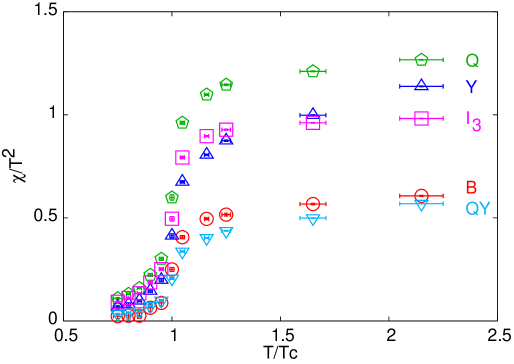
Figure 1: Some of the QNS, $\chi/T^{2}$, as functions of $T/T_{c}$ for $m_{ud}=0.1T_{c}$ and $m_{s}=T_{c}$.

Our primary results for QNS are shown in Figure 1. These were obtained using the eqs. (17) and (19) in Appendix A. The diagonal QNS and several of the off-diagonal ones show the characteristic crossover from small values in the low temperature phase to large values in the high temperature phase which gave rise to the original interpretation that the QCD phase transition liberates quarks milc ; gavai . Observe that $\chi_{B}<\chi_{Q}$ through the full temperature range explored. Both $\chi_{I}$ and $\chi_{Y}$ have values between the two others. In the low temperature phase one has $\chi_{Y}<\chi_{I}$, but for $T\geq 1.5T_{c}$ one obtains $\chi_{Y}>\chi_{I}$. We expect the crossover temperature between these two regimes to vary with quark masses.

Our results are compatible with earlier results with staggered fermions at the same cutoff and quark mass which were obtained in the high temperature phase pushan . They are not directly comparable to results obtained in milc2 at the same lattice spacing due to differences in the discretization.

II.2.1 Robust observables

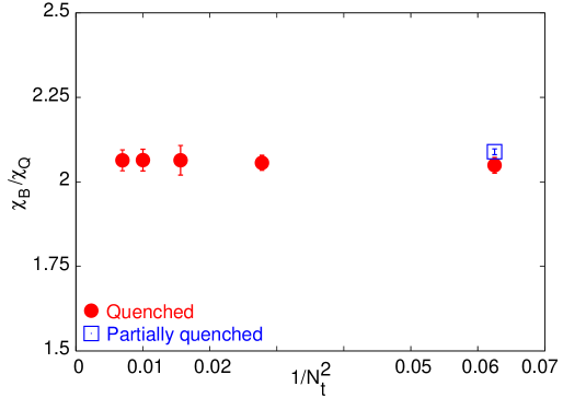
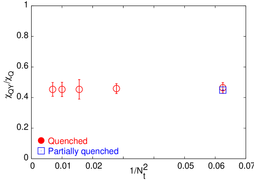
Figure 2: Ratios of QNS are robust observables— being insensitive to both changes in lattice spacing $a\propto 1/N_{t}^{2}$ at fixed $T=2T_{c}$, and the sea quark content of QCD. The quenched results come from a reanalysis of data from conti . In both cases the light valence quark mass is $0.03T_{c}$ and the strange quark mass is $T_{c}$.

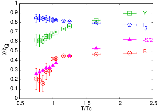
Figure 3: Some robust predictions of fluctuation measures from QCD: all the quantities shown are the ratio $C_{X/Q}$ for the $X$ indicated in the figure, except for $X=S$ which is $C_{S/Q}/2$.

In the quenched theory it was found that the QNS depended quadratically on the lattice spacing conti , i.e., $\chi(a)=\chi+{\cal O}(a^{2})$. Since staggered Fermions have order $a^{2}$ lattice artifacts, one expects the same behaviour in the theory with sea quarks. We are therefore forced to search for observables which are robust against changes in the lattice spacing, in the sense that $r(a)=r+{\cal O}(a^{n})$ with $n>2$. We expect the ratios of QNS to have very good scaling properties in the high temperature phase, where the flavour off-diagonal QNS are much smaller than the flavour diagonal QNS. In the low-temperature phase we do not necessarily expect such behaviour to hold, since these two pieces are comparable, and the coefficient of the order $a^{2}$ corrections in the two parts depend on different physical quantities.

As shown in Figure 2, ratios of QNS in the high temperature phase have this property. The figure also shows another pleasant property— these ratios have little statistically significant dependence on the sea quark content of the theory. We have checked that these two aspects of robustness hold for all ratios in the high temperature phase of QCD. The dependence of such ratios on the valence quark masses can be determined using the quadratic response coefficients (QRC) defined in rajarshi and applied to the study of $C_{B/S}$.

In view of these results, the hierarchy of QNS shown in the previous subsection must be a robust feature of QCD. It is therefore useful to demonstrate this hierarchy by plotting $C_{X/S}$ as a function of $T/T_{c}$ in Figure 3. Our results indicate that experimental studies of $C_{S/Q}$, $C_{B/Q}$ and $C_{Y/Q}$ are the most promising in terms of distinguishing between the two phases of QCD, because they exhibit the largest changes in going from one phase to the other.

II.3 Strange quarks

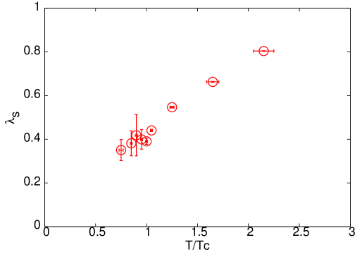
Figure 4: The robust variable $C_{s/u}=\lambda_{s}$ as a function of $T/T_{c}$ when the light quark masses are taken to be $m_{ud}=0.03T_{c}$, corresponding to a realistic pion mass, and the strange quark mass is set to $m_{s}=T_{c}$, which gives a realistic value of the ratio $m_{K}/m_{\pi}$.

The Wroblewski parameter, $\lambda_{s}$, as extracted from experiments, is the ratio of the numbers of primary produced strange and light quark pairs. It has been argued earlier valence that under certain conditions, whose satisfaction can be verified by independent observations, one has $\lambda_{s}=C_{s/u}$. Our results for this robust quantity are shown in Figure 4 prelim . In this computation we have taken the strange quark mass to be $m_{s}=T_{c}$ and the two light quark masses to be degenerate, $m_{ud}=0.03T_{c}$, such that it reproduces the correct value of $m_{\pi}/m_{\rho}$. As can be seen from the figure, the value of the ratio at $T_{c}$ is $\lambda_{s}\approx 0.4$, in agreement with the value of the Wroblewski parameter extracted from experiments, when the freeze-out temperature is close to $T_{c}$ cleymans . It is also a pleasant fact that at lower temperatures the ratio keeps decreasing.

The dependence of this ratio on the valence quark masses was investigated in rajarshi , where it was shown that, in the continuum limit, there was no dependence on valence quark mass except near $T_{c}$. In the vicinity of $T_{c}$, and immediately below, we found $\chi_{s}$ to be strongly dependent on $m_{s}$. It increases as a function of $T/T_{c}$ and at large enough $T$ reaches the same value as $\chi_{u}$, but it does this slowly when $m_{s}/T_{c}$ is large, and faster when $m_{s}\ll T_{c}$. If the plasma contains strange quark quasi-particles, as we argue later, then this behaviour could be a kinematic effect, which measures the phase space for a thermal gluon to split into a strange quark-antiquark pair. That the first effect is dynamical and the second kinematical can be motivated by a study of quantities which vanish in the SU(3) flavour symmetric limit.

II.3.1 Flavour symmetry breaking

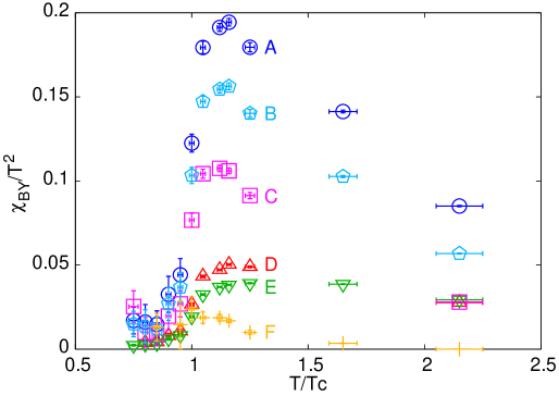
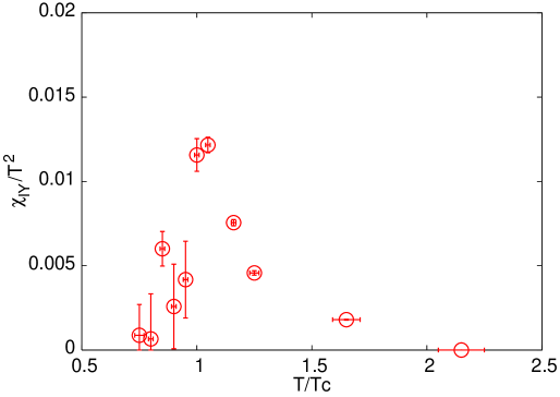
Figure 5: The first panel shows $\chi_{BY}/T^{2}$ as a function of $T/T_{c}$ for various patterns of SU(3) flavour symmetry breaking. Holding $m_{ud}=0.1T_{c}$ constant we vary $m_{s}$ in (A) $m_{s}=T_{c}$, (B) $m_{s}=0.75T_{c}$, and (C) $m_{s}=0.5T_{c}$. Holding $\Delta_{us}=0.25T_{c}$ constant, we vary all the quark masses in (D) $m_{s}=0.75$ and (E) $m_{s}=T_{c}$. In (F) all the quark masses are small $m_{ud}=0.01T_{c}$, $m_{s}=0.1T_{c}$. The second panel shows $\chi_{IY}/T^{2}$, as a function of $T/T_{c}$ when $m_{u}=0.03T_{c}$, $m_{d}=0.1T_{c}$ and $m_{s}=T_{c}$.

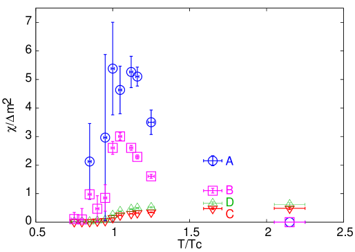
Figure 6: The flavour symmetry breaking matrix elements (A) $\chi_{BY}/\Delta_{us}^{2}$ extracted with $m_{ud}=0.03T_{c}$ and $m_{s}=0.1T_{c}$, and (B) $A_{IY}=\chi_{IY}/\Delta_{ud}^{2}$ extracted using $m_{u}=0.03T_{c}$, $m_{d}=0.1T_{c}$ and $m_{s}=T_{c}$, as a function of $T/T_{c}$. The kinematic suppression for realistic strange quark masses is clear from the significantly smaller values of $\chi_{BY}/\Delta_{us}^{2}$ when (C) $m_{s}=T_{c}$ and (D) $m_{s}=0.75T_{c}$.

Two off-diagonal susceptibilities show an interesting pattern— $\chi_{BQ}$ and $\chi_{BY}$ are both continuous through $T_{c}$, but peak in the vicinity of $T_{c}$. Since $\chi_{BQ}=\chi_{BY}/2$, as seen from eqs. (17) and (19), we show only the latter in Figure (5) for various values of quark masses explained in the caption. The figure also displays $\chi_{IY}$ for $m_{u}\neq m_{d}$. Direct computations also show that $\chi_{BQ}=\chi_{BY}=0$ when all three quark masses are equal, and that $\chi_{IY}=0$ in the SU(2) symmetric limit— providing an explicit demonstration that non-zero values of these quantities are due to flavour symmetry breaking (see the discussion in Appendix A).

From a comparison of the cases (D) and (E) in Figure 5 it is clear that $\chi_{BY}$ is not only a function of $\Delta_{us}=m_{s}-m_{u}$ and $T$ for large values of this asymmetry, since the two curves are not coincident although they have equal $\Delta_{us}$. A careful look at the cases (A), (B) and (C) in the same figure shows that when $m_{s}$ is comparable to $T_{c}$ then both the position and the value of the peak in these QNS are dependent on $m_{s}$. Explicit dependence of the flavour symmetry breaking matrix elements on the actual value of $m_{s}$ (and not just the asymmetry parameter) can only come as a kinematic effect. We try to confirm the magnitude of this effect next.

In Figure 6 we display the values of the dimensionless quantities $A_{IY}=\chi_{IY}/\Delta_{ud}^{2}$ and $A_{BY}=\chi_{BY}/\Delta_{us}^{2}$, extracted using the computations in which $\Delta_{us}$ and $\Delta_{ud}$ are much smaller than $T_{c}$. It would be interesting to check the temperature range in which these dimensionless quantities are computable in weak coupling theory. In the same figure we also show $\chi_{BY}/\Delta_{us}^{2}$ when $\Delta_{us}$ is comparable to $T_{c}$. Its strong suppression relative to the former case shows the kinematic effect which is responsible for the shape of $C_{s/u}$ shown in Figure 4.

The physics of the region just above $T_{c}$ is known to be complicated when observed through gluonic variables such as $\Delta/T^{4}=(\epsilon-3P)/T^{4}$ (where $\epsilon$ is the energy density and $P$ the pressure) as well as the ratio of the lowest lying screening masses in the CP-even and CP-odd sectors saumen . The peaks in $A_{BY}$ and $A_{IY}$ are the first observations of interesting structures near $T_{c}$ in fermionic variables unconnected with the order parameter. It would be interesting to see what temperature range in this is explainable by weak coupling theory.

II.4 Flavour carrying degrees of freedom

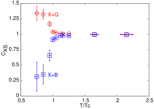
Figure 7: The robust variables $C_{BS}$ and $C_{QS}$, as functions of $T/T_{c}$. The quark masses used are $m_{ud}=0.1T_{c}$ and $m_{s}=T_{c}$, although in the high temperature phase there is no statistically significant dependence on the quark masses.

The question of which are the thermodynamically relevant degrees of freedom in the QCD plasma is easier to answer in the quark sector than in the gluon sector. The reason is that the multitude of flavour quantum numbers allow us to look for “linkage” of flavour, i.e., exciting one quantum number and seeing the magnitude of another quantum number that is simultaneously excited.

II.4.1 Strangeness carriers

Robust variables involving off-diagonal QNS serve precisely this purpose. In koch the robust variable

$$C_{BS}=-3C_{(BS)/S}=-3\,\frac{\chi_{BS}}{\chi_{S}}=1+\frac{\chi_{us}+\chi_{ds}}{\chi_{s}}=1+C_{(us)/s}+C_{(ds)/s}=1+2C_{(us)/s}$$ (4)

is identified as one which can distinguish between bound state QCD bqcd and the usual picture of the excitations in the plasma phase of QCD (in the last expression above we have used eq. (23) and flavour SU(2) symmetry to write $C_{(us)/s}=C_{(ds)/s}$). This is expected to have a value of unity if strangeness is carried by quarks (i.e., $S=1$ always comes linked with $B=-1/3$). In koch it was shown that bound state QGP gives a value of $C_{BS}\approx 2/3$ (for $T>T_{c}$).

We present the first estimate for this quantity from lattice QCD in Figure 7. In the low-temperature phase $C_{BS}$ is very different from unity, but immediately above $T_{c}$ the value is clamped to unity. There is no statistically significant change in $C_{BS}$ as $m_{s}/T_{c}$ is varied between 0.1 and 1. Since the statistical error bars are extremely small for $T\geq T_{c}$, this is a strong statement which contrasts with the $m_{s}$ dependence of $\lambda_{s}$ and $\chi_{BY}$.

Another interesting measure is the correlation of charge and strangeness measured by the robust observable

$$C_{QS}=3C_{(QS)/S}=1-\frac{2\chi_{us}-\chi_{ds}}{\chi_{s}}.$$ (5)

When strangeness is carried by quarks one would expect this to be unity (since $S=1$ comes with $Q=1/3$). In Figure 7 we have also shown the first measurement of $C_{QS}$. Immediately above $T_{c}$ it reaches close to unity with small errors. As a result, these two measurements together quite strongly indicate that unit strangeness is carried by objects with baryon number $-1/3$ and charge $+1/3$ in the high temperature phase of QCD, immediately above $T_{c}$.

Furthermore, eqs. (4, 5) indicate that our observations imply that $\chi_{us}=0$, and hence strangeness carrying excitations do not carry u or d flavour. This is the most direct lattice evidence to date that strangeness is linked to other quantum numbers exactly as it would be for strange quarks, in the high temperature phase of QCD; and that these linkages are quite different below $T_{c}$. Later in this section we show that one should think of these as quasi-particles, dressed by the strong residual interactions, rather than as elementary quarks.

Apart from the direct evidence of linkage between quantum numbers, we also draw attention to the cryptic evidence in the temperature and $m_{s}$ dependence of $C_{BS}$ and $C_{QS}$. The rapid change of $C_{BS}$ with $T$ (for $T<T_{c}$) has a natural explanation if the thermodynamics is controlled by a spectrum of strange baryons such that the amount of (anti-) strangeness per baryon increases with mass, and the masses are larger than $T$. The temperature independence of the two quantities above $T_{c}$ similarly implies that there is one excitation, which has mass less than $T_{c}$. The fact that the values of these quantities do not depend on $m_{s}$ within errors, for $T>T_{c}$, further implies that the effective masses of these quasi-particles is less than $T_{c}$, so that the infrared cutoff on the Dirac operator spectrum is provided by $T$. The next heavier quark, charm quark, does not affect the thermodynamics of the QCD plasma in the range of temperatures we investigate, since its mass is well beyond $T$. However, these heavier quarks do probe changes in other aspects of physics, such as screening, as is evident from jpsi .

II.4.2 The light quark sector

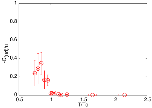
Figure 8: The robust variable $-C_{(ud)/u}$ which measures the correlation between u and d flavours for $m_{ud}=0.1T_{c}$. It is positive in the low temperature phase since u quarks are found along with d antiquarks in charged pions, and vanishes in the high temperature phase, indicating that u and d are fully decorrelated in the plasma. There is no statistically significant dependence on $m_{ud}$ in the high temeperature phase.

In transplanting these methods to the light quark sector, we find that the composite QNS, $\chi_{BI}$ and $\chi_{QI}$, are not informative, since the quark of one flavour has the same isospin as the antiquark of the other flavour. One way to extract information on the degrees of freedom would be to consider QNS of G-parity. However, it is more transparent to turn to the flavoured QNS $\chi_{ud}\propto\langle{\cal N}_{u}{\cal N}_{d}\rangle$. We can then use the quantity

$$C_{(ud)/u}=\frac{\chi_{ud}}{\chi_{u}},$$ (6)

which looks at the linkage between u and d flavours in the same way that $C_{(QS)/S}$ looked for linkage of strangeness and charge. Our results are plotted in the first panel of Figure 8. In the hadronic phase it is non-vanishing because of charged pions, and negative because in these mesons each u comes with a $\overline{\rm d}$, and vice versa. In the QGP phase the vanishing of this normalized covariance implies that a particle with $u$ quantum number does not exhibit $d$ quantum numbers.

Further tests come from investigating

$$C_{(BU)/U} = C_{(BD)/D}=\frac{1}{3}(1+C_{(ud)/u}+C_{(us)/u}),$$

$$C_{(QU)/U} = \frac{1}{3}(2-C_{(ud)/u}-C_{(us)/u}),$$

$$C_{(QD)/D} = -\frac{1}{3}(1-2C_{(ud)/u}+C_{(us)/u}).$$ (7)

The vanishingly small values of $C_{(ud)/u}$ and $C_{(us)/u}$ imply that the u flavour is carried by excitations with baryon number $+1/3$ and charge $+2/3$, whereas the d flavour is carried by particles with baryon number $+1/3$ and charge $-1/3$. These are, therefore, quark quasi-particles.

II.4.3 Quasi-quarks

One might wonder why we talk of, for example, baryon number 1/3 when the measurements even at $2T_{c}$ differ from this number by a few parts in a thousand. What does this small but statistically significant deviation tell us? The answer is that it says something about the spatial structure of the quasi-particle. If flavour were carried by pointlike bare quarks, then $\chi_{ud}$ and $\chi_{us}$ would be precisely zero. However, interactions dress each quark into a spatially extended quasi-particle, and a thermodynamic average probes the spatial dimension of the charge with a resolution of $1/2\pi T$. When $T$ is sufficiently large, so that the gauge coupling is sufficiently small, this structure can be computed in weak coupling theory. As the coupling grows, the perturbative computation fails quantitatively, but as long as the correction to the charge or baryon number remains small, one can fruitfully talk of quasi-quarks.

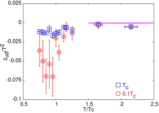
Figure 9: The off-diagonal QNS $\chi_{ud}/T^{2}$ for two different quark masses compared to weak coupling theory. The band includes uncertainties due to neglected of higher loop effects, the effect of changing from one-loop to two-loop computation of the running coupling, and statistical uncertainties in the determination of $T_{c}/\Lambda_{\overline{\scriptscriptstyle MS}}$.

In Figure 9 we show the flavour off-diagonal QNS $\chi_{ud}/T^{2}$ for two different quark masses, along with the prediction of weak coupling perturbation theory bir —

$$\frac{\chi_{ud}}{T^{2}}=-\frac{10}{27\pi^{3}}\alpha_{s}^{3}\log\left(\frac{c}{\alpha_{s}}\right),$$ (8)

where $c$ is a constant whose evaluation requires larger number of loops in the perturbation theory. The strong coupling, $\alpha_{s}$, has been evaluated to two loop accuracy at scale $2\pi T$ with the estimate $T_{c}/\Lambda_{\overline{\scriptscriptstyle MS}}=0.49\pm 0.05$ precise . This variation in $T_{c}/\Lambda_{\overline{\scriptscriptstyle MS}}$, a variation of $c$ by two orders of magnitude, $0.1\leq c\leq 10$, and the variation in $\alpha_{s}$ in going from one loop to the two loop expression are included in the band in the figure. We find that in this range of temperature the prediction is somewhat smaller than the lattice data. Since this is not a robust variable, it is possible that taking the continuum limit will improve the agreement between the two. However, it is clear that as one comes closer to $T_{c}$ the disagreement increases, although the magnitude of $C_{(ud)/u}$ remains small. Thus, it seems that a Fermi gas picture, which may be valid at large $T/T_{c}$, gives way to something more complicated as one approaches $T_{c}$, although the quantum numbers are linked in exactly the same way as for the elementary quarks. This is the meaning of quasi-quarks.

III Summary

We have presented an extensive computation of many different quark number susceptibilities (see Appendix A for the definitions). All the diagonal QNS, and some of the off-diagonal QNS, track the phase structure of QCD— being small in the confined phase and crossing over to larger values in the high temperature phase of QCD, as shown in Figure 1.

An important observation was that ratios of QNS, $C_{A/B}$, defined in eq. (1), are robust variables which depend weakly on the lattice spacing and the sea quark content of QCD in the high temperature phase, as shown in Figure 2. These ratios can be compared to experimentally determined ratios of variances (or covariances) in event-to-event fluctuations of conserved quantum numbers. The relative magnitudes of the diagonal QNS are among these robust observables, and we found the ordering $\chi_{S}>\chi_{Q}>\chi_{Y}>\chi_{I}>\chi_{B}$, shown in Figure 3.

A second set of results concerns the thermal production rate of strange quarks. It has been argued conti that under certain (testable) conditions the Wroblewski parameter is the robust observable $C_{s/u}$. While it is insensitive to the sea quark content of QCD, it is known to depend sensitively on the valence quark masses rajarshi . Here we have determined this quantity for realistic values of the strange and light quark masses (see Figure 4).

We attributed this dependence on $m_{s}$ to kinematic effects visible when $m_{s}\simeq{\cal O}(T_{c})$. However, kinematic effects should manifest themselves in other quantities as well. We tested this hypothesis by examining certain QNS which vanish in the flavour symmetric limit. We extracted the matrix elements which are quadratic in the flavour symmetry breaking mass differences, $\Delta_{us}$, when $\Delta_{us}\ll T_{c}$. By comparing these (in Figure 6) to the corresponding quantities when $\Delta_{us}\approx{\cal O}(T_{c})$, we demonstrated the presence of such kinematic effects in other quantities as well. The flavour symmetry breaking matrix elements themselves (Figure 6) peak at $T$ slighly larger than $T_{c}$, and are the first known example of observables in the quark sector of QCD which parallel similiar structures seen in the gluon sector.

Our final result is that the high temperature phase of QCD essentially consists of quasi-quarks. We demonstrated this by observing that unit strangeness is carried by something which has baryon number $-1/3$ and charge $1/3$, as shown in Figure 7. Part of the argument is that this correlation does not depend on the strange quark mass even when it is as large as $T_{c}$. Similarly, in the light quark sector one finds that u and d quantum numbers are not produced together (Figure 8). Through eqs. (7) we found that this implies that the u flavour is carried by excitations with baryon number $+1/3$ and charge $+2/3$, whereas the d flavour is carried by particles with baryon number $+1/3$ and charge $-1/3$.

We presented an argument that the carriers of these quantum numbers are not elementary quarks but their dressed counterparts which are called quasi-quarks. This argument involved the comparison of $\chi_{ud}$ with a weak-coupling prediction, which is shown in Figure 9. The key point is that this comparison fails badly as one approaches $T_{c}$, although the correlations of flavour quantum numbers remains as they would for quarks. A similar comparison of weak coupling prediction with lattice results for the diagonal QNS $\chi_{u}$ also fails near $T_{c}$, leading us to the same conclusion.

The argument about the existence of quasi-quarks in the high temperature phase of QCD depends on the examination of robust variables given in eq. (3). It is useful to note that their use is not restricted to the lattice. It is also possible to measure them in heavy-ion collisions and thereby deduce the nature of excitations in the fireball produced in these collisions.

We end by pointing out that we have not studied the low-temperature phase of QCD in much detail here. This is an interesting problem, which we have touched upon very briefly in the discussion of $C_{BS}$ and $C_{QS}$, and has been left for the future.

Acknowledgements: This computation was carried out on the Indian Lattice Gauge Theory Initiative’s CRAY X1 at the Tata Institute of Fundamental Research. It is a pleasure to thank Ajay Salve for his administrative support on the Cray. Part of this work was done during a visit under Indo-French (IFCPAR) project, 3104-3 to SPhT, Saclay. The hospitality of Saclay and IFCPAR’s support is gratefully acknowledged.

Appendix A Susceptibilities in equivalent ensembles

Corresponding to every conserved charge, ${\cal Q}$, under the global symmetries of a theory, one can introduce a chemical potential, $\mu$, into thermodynamics, by adding to the action a source term $\mu{\cal Q}$. In QCD, at finite quark mass, one has $SU(N_{f})$ vector flavour symmetry. Corresponding to each of the $N_{f}$ flavours, one can introduce a chemical potential $\mu_{f}$ ($f=u$, $d$, $s$, etc.) through the term

$$J=\sum_{f}\mu_{f}{\cal N}_{f}=\mu^{T}{\cal N},$$ (9)

where ${\cal N}_{f}$ is the number operator for quarks of flavour $f$, whose expectation value is the number of quarks minus the number of antiquarks. The last expression just rewrites the sum as a dot product of the vector of intensive variables $\mu$ with the vector of extensive variables ${\cal N}$. This corresponds to a grand canonical ensemble in which the chemical potential on each of the quark flavours can be tuned independently. In the corresponding canonical ensemble the number of quarks of each flavour is kept fixed.

The number densities, which are the first derivative of the pressure with respect to the chemical potential, and the quark number susceptibilities (QNS), which are the second derivatives, have been defined before milc ; conti . Here we use the notation of conti for the QNS. We shall also use a higher order susceptibility, for which we use the notation of endpt .

It is usually more convenient to define chemical potentials for variables which are easier to control in experiments— such as the baryon number, $B$, the electric charge, $Q$, the third component of isospin, $I_{3}$, or the hypercharge, $Y$. Any choice of $N_{f}$ variables corresponds to a different choice of ensemble to describe the same physics. The description in terms of flavours given above can then be translated into the new ensemble by a simple linear transformation

$$J=\mu^{T}M^{-1}M{\cal N}=(\mu^{\prime})^{T}{\cal N}^{\prime},\qquad i.e.,\qquad{\cal N}^{\prime}=M{\cal N}\quad{\rm and}\quad\mu^{\prime}=(M^{-1})^{T}\mu=(M^{T})^{-1}\mu.$$ (10)

Clearly, the partition function being the same, the physics remains invariant under these redefinitions. The choice of a given $M$ corresponds to putting coordinates in Gibbs space.

One is usually interested in thermodynamics quantities or response functions which are obtained by taking derivatives of the free energy or pressure with respect to the chemical potentials. Note that by the definitions in eq. (10), one has $\mu=M^{T}\mu^{\prime}$. The chain rule for differentiation then tells us that

$$\frac{\partial}{\partial\mu^{\prime}_{i}}=\frac{\partial\mu_{j}}{\partial\mu^{\prime}_{i}}\frac{\partial}{\partial\mu_{j}}=(M^{T})_{ji}\frac{\partial}{\partial\mu_{j}}=M_{ij}\frac{\partial}{\partial\mu_{j}}$$ (11)

The fact that this gives back the original definitions of the ${\cal N}^{\prime}$s in terms of the ${\cal N}$s is a consistency check of the formalism. We illustrate the uses of this formalism for the cases of $N_{f}=2$ and $N_{f}=3$ below.

A.1 $N_{f}=2$

A.1.1 The $B$, $I_{3}$ ensemble

In the two flavour case, one can transform from the flavour basis to the set

$$B=\frac{1}{3}({\cal N}_{u}+{\cal N}_{d}),\qquad \mu_{B}=\frac{3}{2}(\mu_{u}+\mu_{d}),$$

$$I_{3}=\frac{1}{2}({\cal N}_{u}-{\cal N}_{d}),\qquad \mu_{I}=\mu_{u}-\mu_{d}.$$ (12)

Inverting the relation between chemical potentials one obtains $\mu_{u}=\mu_{B}/3+\mu_{I}/2$ and $\mu_{d}=\mu_{B}/3-\mu_{I}/2$. In the ensemble where $\mu_{I}=0$, one then gets $\mu_{u}=\mu_{d}=\mu_{B}/3$. The number densities are given by eq. (12). The quark number susceptibilities are—

$$\chi_{B} = \frac{1}{9}(\chi_{uu}+\chi_{dd}+2\chi_{ud})=\frac{2}{9}(\chi_{u}+\chi_{ud}),$$

$$\chi_{I} = \frac{1}{4}(\chi_{uu}+\chi_{dd}-2\chi_{ud})=\frac{1}{2}(\chi_{u}-\chi_{ud}),$$

$$\chi_{BI} = \frac{1}{6}(\chi_{uu}-\chi_{dd})=0,$$ (13)

where the first expression in each case is the most general, and the second is obtained for exact vector SU(2) flavour symmetry $m_{ud}$. If this symmetry is broken then $\chi_{BI}$ should become non-zero. For small values of the symmetry breaking parameter $\Delta_{ud}=m_{d}-m_{u}$ (we will follow the convention that $m_{u}\leq m_{d}\leq m_{s}$),

$$\chi_{BI}=A_{BI}\Delta_{ud}^{2},\qquad{\rm which\ yields}\qquad\frac{\chi_{BI}}{T_{c}^{2}}=A_{BI}\left(\frac{\Delta_{ud}}{T_{c}}\right)^{2},$$ (14)

where $A_{BI}$ is a dimensionless number. We present results for this quantity in Figure 6. In the low temperature phase we expect that $A_{BI}$ is a non-perturbative quantity, but that it should be computable in chiral perturbation theory. It would be interesting to check how far the weak coupling theory in the high temperature phase agrees with our determination of $A_{BI}$.

A.1.2 The $B$, $Q$ ensemble

One may choose to work in another ensemble given by

$$B=\frac{1}{3}({\cal N}_{u}+{\cal N}_{d}),\qquad \mu_{B}=\mu_{u}+2\mu_{d},$$

$$Q=\frac{1}{3}(2{\cal N}_{u}-{\cal N}_{d}),\qquad \mu_{Q}=\mu_{u}-\mu_{d}.$$

For $\mu_{Q}=0$, one gets again the expected result $\mu_{u}=\mu_{d}=\mu_{B}/3$. The quark number susceptibilities in this ensemble are—

$$\chi_{B} = \frac{1}{9}(\chi_{uu}+\chi_{dd}+2\chi_{ud})=\frac{2}{9}(\chi_{u}+\chi_{ud}),$$

$$\chi_{Q} = \frac{1}{9}(4\chi_{uu}+\chi_{dd}-4\chi_{ud})=\frac{1}{9}(5\chi_{u}-4\chi_{ud}),$$

$$\chi_{BQ} = \frac{1}{9}(2\chi_{uu}-\chi_{dd}+\chi_{ud})=\frac{1}{9}(\chi_{u}+\chi_{ud}),$$ (15)

where the last expression in each line holds in the special case of $m_{ud}$. Note that $\chi_{BB}$ is the same in both the ensembles. This follows from the fact that the definition of the baryon number is the same.

A.2 $N_{f}=3$

A.2.1 The $B$, $I_{3}$, $Y$ ensemble

The variables in this ensemble are

$$B=\frac{1}{3}({\cal N}_{u}+{\cal N}_{d}+{\cal N}_{s}),\qquad \mu_{B}=\mu_{u}+\mu_{d}+\mu_{s},$$

$$I_{3}=\frac{1}{2}({\cal N}_{u}-{\cal N}_{d}),\qquad \mu_{I}=\mu_{u}-\mu_{d},$$

$$Y=\frac{1}{3}({\cal N}_{u}+{\cal N}_{d}-2{\cal N}_{s}) \mu_{Y}=\frac{1}{2}(\mu_{u}+\mu_{d}-2\mu_{s}).$$ (16)

The six independent quark number susceptibilities are

$$\chi_{B} = \frac{1}{9}(\chi_{u}+\chi_{d}+\chi_{s}+2\chi_{ud}+2\chi_{us}+2\chi_{ds})=\frac{1}{9}(2\chi_{u}+\chi_{s}+2\chi_{ud}+4\chi_{us}),$$

$$\chi_{I} = \frac{1}{4}(\chi_{u}+\chi_{d}-2\chi_{ud})=\frac{1}{2}(\chi_{u}-\chi_{ud}),$$

$$\chi_{Y} = \frac{1}{9}(\chi_{u}+\chi_{d}+4\chi_{s}+2\chi_{ud}-4\chi_{us}-4\chi_{ds})=\frac{2}{9}(\chi_{u}+2\chi_{s}+\chi_{ud}-4\chi_{us}),$$

$$\chi_{BI} = \frac{1}{6}(\chi_{u}-\chi_{d}+\chi_{us}-\chi_{ds})=0,$$

$$\chi_{BY} = \frac{1}{9}(\chi_{u}+\chi_{d}-2\chi_{s}+2\chi_{ud}-\chi_{us}-\chi_{ds})=\frac{2}{9}(\chi_{u}-\chi_{s}+\chi_{ud}-\chi_{us}),$$

$$\chi_{IY} = \frac{1}{9}(\chi_{u}-\chi_{d}-2\chi_{us}+2\chi_{ds})=0.$$ (17)

As before, the last set of expressions on each line holds only for $m_{ud}\neq m_{s}$. Similiar to eq. (14), one can define $A_{BI}$ here, and also $A_{IY}=\chi_{IY}/\Delta_{ud}^{2}$, both of which are generally non-vanishing when SU(2) flavour symmetry is broken.

In the SU(3) symmetric limit, $m_{u}=m_{d}=m_{s}$, the three off-diagonal susceptibilities vanish, i.e., $\chi_{BI}=\chi_{BY}=\chi_{IY}=0$. Also, in this limit one has $2\chi_{I}=3\chi_{Y}/2=\chi_{u}-\chi_{ud}$ and $3\chi_{B}=\chi_{u}+2\chi_{ud}$. In the low temperature phase the breaking of vector SU(3) symmetry produces the mass difference between the pion and the K meson. At sufficiently high temperature, when the strange quark mass is less than the Matsubara frequency, $m_{s}<2\pi T$, the theory becomes effectively SU(3) symmetric, and the above relations should hold. In the high temperature phase of QCD one also has $\chi_{ud}\propto g^{5}\log g\to 0$ bir , so one should obtain $2\chi_{I}=3\chi_{Y}/2=3\chi_{B}$.

A.2.2 The $B$, $Q$, $Y$ ensemble

Another useful set of charges and associated chemical potentials is

$$B=\frac{1}{3}({\cal N}_{u}+{\cal N}_{d}+{\cal N}_{s}),\qquad \mu_{B}=\mu_{u}+\mu_{d}+\mu_{s},$$

$$Q=\frac{1}{3}(2{\cal N}_{u}-{\cal N}_{d}-{\cal N}_{s}),\qquad \mu_{Q}=\mu_{u}-\mu_{d},$$

$$Y=\frac{1}{3}({\cal N}_{u}+{\cal N}_{d}-2{\cal N}_{s}),\qquad \mu_{Y}=\mu_{d}-\mu_{s}.$$ (18)

The three susceptibilities $\chi_{B}$, $\chi_{Y}$ and $\chi_{BY}$ are the same as in the previous ensemble. The remaining susceptibilities are

$$\chi_{Q} = \frac{1}{9}(4\chi_{u}+\chi_{d}+\chi_{s}-4\chi_{ud}-4\chi_{us}+2\chi_{ds})=\frac{1}{9}(5\chi_{u}+\chi_{s}-4\chi_{ud}-2\chi_{us}),$$

$$\chi_{BQ} = \frac{1}{9}(2\chi_{u}-\chi_{d}-\chi_{s}+\chi_{ud}+\chi_{us}-2\chi_{ds})=\frac{1}{9}(\chi_{u}-\chi_{s}+\chi_{ud}-\chi_{us}),$$

$$\chi_{QY} = \frac{1}{9}(2\chi_{u}-\chi_{d}+2\chi_{s}+\chi_{ud}-5\chi_{us}+\chi_{ds})=\frac{1}{9}(\chi_{u}+2\chi_{s}+\chi_{ud}-4\chi_{us}).$$ (19)

As before, the last set of expressions on each line holds only for $m_{ud}\neq m_{s}$. Note that in this limit one has $\chi_{BQ}=\chi_{BY}/2$.

In the SU(3) symmetric limit, $m_{ud}=m_{s}$, two of the off-diagonal susceptibilities vanish, i.e., $\chi_{BQ}=\chi_{BY}=0$. Also, in this limit one has $\chi_{Q}=\chi_{Y}=2\chi_{QY}=2(\chi_{u}-\chi_{ud})/3$ and $\chi_{B}=(\chi_{u}+2\chi_{ud})/3$. As before, in the high temperature limit, when the quark masses are less than the temperature, the theory becomes effectively SU(3) symmetric. Then taking $\chi_{ud}=0$, one should obtain $\chi_{Q}=\chi_{Y}=2\chi_{B}=2\chi_{QY}$.

It is interesting to examine this in a theory of massless free fermions. The free energy is given by

$$F=N_{c}V\sum_{f=u,d,s}\left[\frac{7\pi^{2}}{180}T^{4}+\frac{1}{6}\mu^{2}T^{2}+\frac{1}{12\pi^{2}}\mu^{4}\right].$$ (20)

Substituting the values of the flavour chemical potential by the appropriate combination of $\mu_{B}$, $\mu_{Q}$ and $\mu_{Y}$, and taking the derivatives, we find that $\chi_{BY}=\chi_{BQ}=0$. Also, $\chi_{Q}=\chi_{Y}=2\chi_{B}=2\chi_{QY}=2N_{c}/9$. For massive free fermions, when $T$ is much larger than the fermion mass, the same results would hold.

When SU(3) symmetry is broken through the parameter $\Delta_{us}=m_{s}-m_{u}$ (we assume that SU(2) symmetry still holds) then for small $\Delta_{us}$ one may again write

$$\chi_{BY}=A_{BY}\Delta_{us}^{2}\qquad{\rm and}\qquad\chi_{BQ}=A_{BQ}\Delta_{us}^{2}.$$ (21)

As before, we expect $A_{BY}$ and $A_{BQ}$ to be non-perturbative but computable in chiral perturbation theory in the low temperature phase. It would be interesting to compare our results (presented later) with weak coupling theory in the high temperature phase.

A.2.3 The $B$, $Q$, $S$ ensemble

From the experimental point of view, it may be interesting to use the set

$$B=\frac{1}{3}({\cal N}_{u}+{\cal N}_{d}+{\cal N}_{s}),\qquad \mu_{B}=\mu_{u}+2\mu_{d},$$

$$Q=\frac{1}{3}(2{\cal N}_{u}-{\cal N}_{d}-{\cal N}_{s}),\qquad \mu_{Q}=\mu_{u}-\mu_{d},$$

$$S=-{\cal N}_{s},\qquad \mu_{S}=\mu_{d}-\mu_{s}.$$ (22)

Note that we have used the standard convention where the strangeness of the antistrange quark is $+1$. The three susceptibilities, $\chi_{B}$, $\chi_{Q}$ and $\chi_{BQ}$ are as before. The remainder are

$$\chi_{S} = \chi_{s},$$

$$\chi_{BS} = -\frac{1}{3}(\chi_{s}+\chi_{us}+\chi_{ds})=-\frac{1}{3}(\chi_{s}+2\chi_{us}),$$

$$\chi_{QS} = \frac{1}{3}(\chi_{s}-2\chi_{us}+\chi_{ds})=\frac{1}{3}(\chi_{s}-\chi_{us}).$$ (23)

As always, the last set of expressions on each line holds only for $m_{ud}\neq m_{s}$.

A.2.4 The $B$, $Q$, $U$ ensemble

For technical questions about the light quark sector it is useful to work in the ensemble with

$$B = \frac{1}{3}({\cal N}_{u}+{\cal N}_{d}+{\cal N}_{s}),$$

$$Q = \frac{1}{3}(2{\cal N}_{u}-{\cal N}_{d}-{\cal N}_{s}),$$

$$U = {\cal N}_{u},$$ (24)

The three susceptibilities, $\chi_{B}$, $\chi_{Q}$ and $\chi_{BQ}$ are as before. The rest are

$$\chi_{U} = \chi_{u},$$

$$\chi_{BU} = \frac{1}{3}(\chi_{u}+\chi_{ud}+\chi_{us}),$$

$$\chi_{QU} = \frac{1}{3}(2\chi_{u}-\chi_{ud}-\chi_{us}).$$ (25)

Changing to an ensemble where $U$ is replaced by $D={\cal N}_{d}$ changes the QNS to

$$\chi_{D} = \chi_{u},$$

$$\chi_{BD} = \frac{1}{3}(\chi_{u}+\chi_{ud}+\chi_{us}),$$

$$\chi_{QD} = -\frac{1}{3}(\chi_{u}-2\chi_{ud}+\chi_{us}),$$ (26)

where we have used SU(2) symmetry. This gives $\chi_{U}=\chi_{D}$ and $\chi_{BU}=\chi_{BD}$.

References

- (1) M. Asakawa, U. Heinz and B. Muller, Phys. Rev. Lett. 85, 2072 (2000).
- (2) S.-Y. Jeon and V. Koch, Phys. Rev. Lett. 85, 2076 (2000).
- (3) C. Pruneau, S. Gavin and S. Voloshin, nucl-ex/0204011.
- (4) K. D. Born et al., Phys. Rev. Lett. 67 302 (1991).
- (5) R. V. Gavai and S. Gupta, Phys. Rev. D 67, 034501 (2003).
- (6) J.-P. Blaizot, E. Iancu and A. Rebhan, Phys. Lett. B 523, 143 (2001).
- (7) A. Vuorinen, Phys. Rev. D 68, 054017 (2003).
- (8) R. V. Gavai, S. Gupta and P. Majumdar, Phys. Rev. D 65, 054506 (2002).
- (9) V. Koch, A. Majumder and J. Randrup, nucl-th/0505052.
- (10) L. D. Landau and E. M. Lifschitz, Statistical Mechanics, 3rd enlarged edition, Pergamon Press, Oxford, England (1986).
- (11) R. V. Gavai and S. Gupta, Phys. Rev. D 64, 074506 (2001).
- (12) R. V. Gavai and S. Gupta, Phys. Rev. D 71, 114014 (2005).
- (13) R. V. Gavai and S. Gupta, Phys. Rev. D 72, 054006 (2005).
- (14) S. Gottlieb et al., Phys. Rev. Lett. 59, 2247 (1987).
- (15) R. V. Gavai, J. Potvin and S. Sanielevici, Phys. Rev. D 40, 2743 (1989).
- (16) C. Bernard et al., Phys. Rev. D71, 034504 (2005).
- (17) R. V. Gavai and S. Gupta, Phys. Rev. D 65, 094515 (2002).
- (18) S. Gupta and R. Ray, Phys. Rev. D 70, 114015 (2004).
- (19) R. V. Gavai and S. Gupta, J. Phys. G 30, S1333 (2004) contains a preliminary version of these results.
- (20) J. Cleymans, J. Phys. G 28, 1575 (2002).
- (21) S. Dutta and S. Gupta, Phys. Rev. D 67, 054503 (2003).
- (22) E. V. Shuryak and I. Zahed, Phys. Rev. D 70, 054507 (2004).
-
(23)
M. Asakawa and T. Hatsuda, Phys. Rev. Lett. 92, 012001 (2004);
S. Datta et al., Phys. Rev. D 69, 094507 (2004). - (24) S. Gupta, Phys. Rev. D 64, 034507 (2001).