A new efficient Cluster Algorithm for the Ising Model

Abstract:

Using D-theory we construct a new efficient cluster algorithm for the Ising model. The construction is very different from the standard Swendsen-Wang algorithm and related to worm algorithms. With the new algorithm we have measured the correlation function with high precision over a surprisingly large number of orders of magnitude.

PoS(LAT2005)112

1 Reformulation of the Ising Model

D-theory [1] is an alternative way of regularising field theories by dimensional reduction of systems involving discrete variables, that allows us to develop cluster algorithms. One can also use this method to describe and simulate a simple spin system such as the Ising model. Besides being interesting in its own right, we hope to gain some insights that may be useful for the construction of cluster algorithms for gauge theories.

We consider the Ising model with the classical Hamilton function ${\cal H}[s]=-J\sum_{x,\mu}s_{x}s_{x+\hat{\mu}}$, and rewrite it as a quantum system with the Hamiltonian $H=-J\sum_{x,\mu}\sigma_{x}^{3}\sigma_{x+\hat{\mu}}^{3}$. Due to the trace-structure of the partition function, $Z=\mbox{Tr}\exp(-\beta H)$, we can perform a unitary transformation rotating to a basis containing $\sigma^{1}$:

$$H=-J\sum_{x,\mu}\sigma_{x}^{1}\sigma_{x+\hat{\mu}}^{1}.$$ (1)

We then perform a Trotter decomposition of the Hamiltonian. In one dimension this implies the following splitting into two parts,

$$H=H_{1}+H_{2},\ H_{1}=-J\sum_{x\ even}\sigma_{x}^{1}\sigma_{x+1}^{1},\ H_{2}=-J\sum_{x\ odd}\sigma_{x}^{1}\sigma_{x+1}^{1},$$ (2)

while in two dimensions one needs four parts

$$H_{1}=\sum_{x\in(2m,n)}h_{x,\hat{1}},\ H_{2}=\sum_{x\in(m,2n)}h_{x,\hat{2}},\ H_{3}=\sum_{x\in(2m+1,n)}h_{x,\hat{1}},\ H_{4}=\sum_{x\in(m,2n+1)}h_{x,\hat{2}}.$$ (3)

The partition function can then be turned into a path integral with $M$ time steps of width $\epsilon$ ($\beta=\epsilon M$). The Euclidean time serves as an additional dimension whose extent $\beta$ determines the inverse temperature. For example in the 1-dimensional Ising model, the Trotter decomposition of the partition function takes the form

$$Z=\mbox{Tr}\exp(-\epsilon H_{1}-\epsilon H_{2})^{M}=\mbox{Tr}\exp(-\epsilon H_{1})^{M}\exp(-\epsilon H_{2})^{M}.$$ (4)

In this way we obtain a checkerboard decomposition where the action resides on the shaded plaquettes (see figure 1).

\psfrag{b=eM}{$\beta=\epsilon M$}\psfrag{e}{$\epsilon$}\psfrag{T}{$T$}\psfrag{x}{$x$}\includegraphics[height=99.58464pt]{trotter2d.eps}

Figure 1: Trotter decomposition in one dimension with a spin-configuration: crosses and circles represent the two spin states.

In general the Trotter decomposition is affected by an order $\epsilon^{2}$ error. However, since in the Ising model $H_{1}$ and $H_{2}$ commute, it is an exact rewriting of the partition function and even with the minimal number of time-slices one obtains the continuous time limit.

2 Construction of the Algorithm

In our basis the transfer matrix of a single plaquette $T=\exp(-\epsilon\sigma_{x}^{1}\sigma_{x+1}^{1})$ takes the form

$${T=\small\begin{array}[]{cc}\begin{array}[]{cccc}\uparrow\uparrow&\uparrow\downarrow&\downarrow\uparrow&\downarrow\downarrow\end{array}&\\ \left(\begin{array}[]{cccc}c&0&0&s\\ 0&c&s&0\\ 0&s&c&0\\ s&0&0&c\end{array}\right)&\begin{array}[]{c}\uparrow\uparrow\\ \uparrow\downarrow\\ \downarrow\uparrow\\ \downarrow\downarrow\\ \end{array}\end{array}},$$ (5)

with $c=\cosh(\epsilon J)$ and $s=\sinh(\epsilon J)$. From this we can see that there are only eight physically allowed plaquette configurations (see figure 3).

In order to imply constraints on the relative orientation of the spins on a plaquette, we propose plaquette breakups that bind spins together. These constraints must be maintained in the cluster update. The breakups give rise to clusters and these clusters can only be flipped as a whole. In this way, by construction, one indeed maintains the constraints implied by the cluster breakups. We choose to use the $A$, $B_{1}$, and $B_{2}$ breakups shown in figure 3.

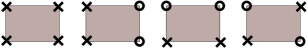
Figure 2: Allowed plaquettes.

\psfrag{A}{$A$}\psfrag{B1}{$B_{1}$}\psfrag{B2}{$B_{2}$}\includegraphics[height=25.6073pt]{breakups.eps}

Figure 3: Cluster breakups.

These breakups decompose the transfer matrix as follows:

$$T=A\left({\scriptsize\begin{array}[]{cccc}1&0&0&0\\ 0&1&0&0\\ 0&0&1&0\\ 0&0&0&1\\ \end{array}}\right)+B_{1}\left({\scriptsize\begin{array}[]{cccc}1&0&0&1\\ 0&0&0&0\\ 0&0&0&0\\ 1&0&0&1\\ \end{array}}\right)+B_{2}\left({\scriptsize\begin{array}[]{cccc}0&0&0&0\\ 0&1&1&0\\ 0&1&1&0\\ 0&0&0&0\\ \end{array}}\right).$$ (6)

From eq.(5), one obtains $B_{1}=B_{2}=s$ and $A=c-s$. Using these cluster breakups we can now simulate the system. In figure 4 we show an example of a cluster update in which the dashed cluster has been flipped.

$\begin{array}[]{lll}\includegraphics[height=85.35826pt]{cluster_0.eps}&&\includegraphics[height=85.35826pt]{cluster2_0.eps}\end{array}$

Figure 4: A configuration with $A$, $B_{1}$, and $B_{2}$ breakups with a multi-cluster update.

The energy density is related to the fraction $P$ of interaction plaquettes with a transition (spins opposite in time on a plaquette) by the equation

$$E=\langle H\rangle=-J(t+\frac{(1-t^{2})}{t}\langle P\rangle),$$ (7)

where $t=\tanh(\epsilon J)$.

Analysing the average cluster-size of the algorithm in multi-cluster mode shows that it is indeed very different from the Swendsen-Wang algorithm [2]. In two dimensions, with the Trotter decomposition of eq.(3) and the minimal number of four time-slices, we observe a peak at the critical temperature, whereas Swendsen-Wang clusters still grow in the broken phase. This is shown in figure 5.

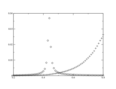
Figure 5: Average cluster-size of the new algorithm (diamonds) compared to the Swendsen-Wang algorithm (crosses) on a $100^{2}$ lattice.

3 Measurement of the 2-Point Correlation Function

The correlation function is defined in our basis as $\langle\sigma^{1}_{0}\sigma^{1}_{x}\rangle$. The $\sigma^{1}$ matrices are off-diagonal and flip the spins they act on. Thus they can be viewed as violations of spin conservation, i.e. two opposite spins reside on the same site (see figure 6).

$\begin{array}[]{ccc}\sigma^{1}={\small\begin{array}[]{cc}\begin{array}[]{cc}\uparrow&\downarrow\end{array}&\\ \left(\begin{array}[]{cc}0&1\\ 1&0\end{array}\right)&\begin{array}[]{c}\uparrow\\ \downarrow\end{array}\end{array}}&&\begin{array}[]{c}\\ \includegraphics[height=34.14322pt]{violation.eps}\end{array}\end{array}$

Figure 6: The action of the operator $\sigma^{1}$ on a site, seen as a violation of spin conservation.

What we do is the following: we introduce two violations on a random site (where they cancel each other), build the clusters, and flip them with probability $p=\frac{1}{2}$, unless it is a cluster with one or two violations. There we flip a fraction of the cluster in order to move the violations to different positions. For example in figure 7, the dashed part of a cluster with violations has been flipped.

\psfrag{A}{$A$}\psfrag{B1}{$B_{1}$}\psfrag{B2}{$B_{2}$}\includegraphics[height=85.35826pt]{cluster.eps}

\psfrag{A}{$A$}\psfrag{B1}{$B_{1}$}\psfrag{B2}{$B_{2}$}\includegraphics[height=85.35826pt]{cluster2.eps}

Figure 7: Partially flipping a cluster with violations (circles).

When the violations are on the same site, we introduce them randomly somewhere else. By histogramming the spatial distance between the two violations, we get a very accurate measurement of the correlation function. One then normalises the correlation function to 1 at zero distance. In figure 10 this is compared to the analytic result [3].

4 Improved Estimator for the Susceptibility

The susceptibility can be measured by summing over the correlation function. This is already an improved estimator because one gets only positive contributions. One can also measure the average frequency of reaching spatial distance zero. This corresponds to the inverse susceptibility. In a large system at high temperature this is not too efficient yet and can be further improved.

We project the clusters with violations to the spatial volume and measure their overlap. This gives us the probability that two violations are at zero spatial distance in the next cluster update and, again, corresponds to measuring the inverse susceptibility. In this way we gain statistics by a factor of the cluster-size squared $|C|^{2}$ with an effort proportional to the cluster-size $|C|$.

5 Worm-Algorithm

Instead of using clusters, we can — with the same breakups — move the two violations locally with a worm-type Metropolis algorithm [4].

\psfrag{b=eM}{$\beta=\epsilon M$}\psfrag{e}{$\epsilon$}\psfrag{T}{$T$}\psfrag{x}{$x$}\includegraphics[height=85.35826pt]{worm.eps}

Figure 8: Worm moving the violations and thus updating a given configuration.

Interestingly we can also measure n-point functions by introducing $n$ violations. These violations are moved in the same way as above.

5.1 Snake-Algorithm — Improved Correlation Function Measurement

An efficient trick [5] allows us to measure an exponentially suppressed signal with a linear effort. The correlation function is exponentially suppressed in the high-temperature phase and is thus hard to measure at large distances. The correlation function is the ratio of two partition functions and it can be rewritten as the product of many fractions which can be measured individually:

$$\langle\sigma_{0}^{1}\sigma_{x}^{1}\rangle=\frac{Z(x)}{Z(0)}=\frac{Z(1)}{Z(0)}\frac{Z(2)}{Z(1)}\dots\frac{Z(x)}{Z(x-1)}.$$ (8)

In figure 10 we compare the numerical results at very high temperature with the analytical expression [3].

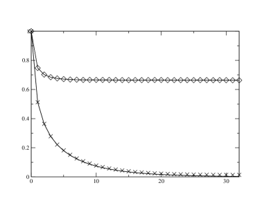
Figure 9: Correlation function on a $64^{2}$-lattice at $\beta=0.42$ (crosses) and $\beta=0.46$ (diamonds) compared to the analytic result.

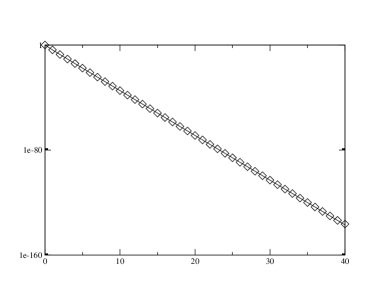
Figure 10: Correlation function on an $80^{2}$-lattice at $\beta=0.01$.

6 Conclusion

Using D-theory we have constructed a new efficient algorithm for the Ising model. We have an improved estimator for the susceptibility. Combining the algorithm with the snake algorithm one can measure the correlation function in regions otherwise hardly accessible. We would like to apply this approach to other theories, possibly gauge theories.

References

- [1] R. Brower, S. Chandrasekharan, S. Riederer, and U. J. Wiese, Nucl. Phys. B 693 (2004) 149 [arXiv:hep-lat/0309182].
- [2] R. H. Swendsen and J. S. Wang, Phys. Rev. Lett. 58 (1987) 86.
- [3] M. Jimbo and T. Miwa, Proc. Japan Acad. A 56 (1980) 405-410, Errata 57 (1981) 347.
- [4] N. Prokof’ev and B. Svistunov, Phys. Rev. Lett. 87 (2001) 160601 [arXiv:cond-mat/0103146].
- [5] P. de Forcrand, M. D’Elia and M. Pepe, Phys. Rev. Lett. 86 (2001) 1438 [arXiv:hep-lat/0007034].