Perturbative Study of the Supersymmetric Lattice Model from Matrix Model

Abstract:

We study the lattice model for the supersymmetric Yang-Mills theory in two dimensions proposed by Cohen, Kaplan, Katz, and Unsal. We re-examine the formal proof for the absence of susy breaking counter terms as well as the stability of the vacuum by an explicit perturbative calculation for the case of $U(2)$ gauge group. Introducing fermion masses and treating the bosonic zero momentum mode nonperturbatively, we avoid the infra-red divergences in the perturbative calculation. As a result, we find that there appear mass counter terms for finite volume which vanish in the infinite volume limit so that the theory needs no fine-tuning.

PoS(LAT2005)271

1 Introduction

Cohen-Kaplan-Katz-Unsal(CKKU) [1],[2] model is one of the promising formulations of the supersymmetric gauge theories without fine-tuning [3]. Their model is constructed from matrix model by using orbifolding [4] and deconstruction [5], where the lattice spacing is dynamically obtained as the inverse vacuum expectation value of the scalar degrees of freedom in the matrix mode.

One possible problem in CKKU model is that the extended supersymmetry has flat directions for the scalar so that the lattice structure from the deconstruction suffers from the instability due to the quantum fluctuations of the scalar zero momentum modes. To suppress the divergence in the flat directions, soft susy-breaking terms for the scalar fields are introduced. Since such terms break the supersymmetry and cause the infra-red divergence, the original discussion of the renormalization based on exact supersymmetry on the lattice has to be modified by including the breaking terms. It is therefore important to re-examine the renormalization at 1-loop level by explicit calculations in order to see whether this theory really needs fine-tuning or not.

2 Method for perturbative calculation

2.1 Counter terms

Before explaining our calculational method, let us discuss possible counter terms which needs renormalization. Radiative corrections induce the operator $\mathcal{O}$ of the following structure into the action

$$\delta S=\frac{1}{g_{2}^{2}}Tr\int d^{2}z\mathcal{C_{O}}\mathcal{O}.$$ (1)

Relevant or marginal operators ($\mathcal{O}$) whose canonical dimension $M[\mathcal{O}]=p$ at the $l$-loop correction must satisfy

$$p\leq 4-2l$$ (2)

At 1-loop level, relevant or marginal operators with dimensions $0\leq p\leq 2$ can arise. At 2-loop level, relevant operators with the dimension $p=0$ can arise. Beyond 2-loop, there is no relevant or marginal counter term. Since the operator with the dimension $p=0$ is the cosmological constant, it does not play any serious role in fine-tuning problems.

Let us now focus on the 1-loop relevant or marginal counter-terms. Since bosonic fields have dimension 1 and fermionic fields have dimension $\frac{3}{2}$, the candidates for such operators are bosonic 1-point and 2-point functions. Although fermionic 1-point functions are possible from dimension counting, they are forbidden by Grassman parity.

Since 1-point functions of gauge fields are forbidden from Furry’s theorem and the 2-point ones are also forbidden by the gauge symmetry. Hence the only possible counter terms are

• $<s_{x}>,<s_{y}>$ (scalar 1point functions),

• $<s^{2}_{x}>,<s^{2}_{y}>$ (scalar 2point functions).

In what follows, we will discuss the renormalization of these two operators.

2.2 Calculational method for treating infra-red problems from fermion and bosons

Let us explain the infra-red divergence problem from fermions and bosons. It was pointed out by Giedt [6] that there exists an exact zero mode of the fermion matrix called ‘ever-existing zero mode’. Since it completely decouples from the action the fermion path-integral over this mode is ill-defined. Since there is no kinetic term for the zero momentum mode for the gauge field perturbative calculations based on the gaussian integral are also ill-defined.

In order to make the fermion path-integral well-defined we propose to introduce the fermion mass term with coefficient $\mu_{F}$ inversely proportional to the lattice size $L$ to the action as

$$S_{2} = S_{1}+\frac{a\mu_{F}\sqrt{2}}{g^{2}}Tr\sum_{\mathbf{n}}(\alpha_{\mathbf{n}}\bar{x}_{\mathbf{n}}\lambda_{\mathbf{n}}+\beta_{\mathbf{n}}\bar{y}_{\mathbf{n}}\lambda_{\mathbf{n}}-\alpha_{\mathbf{n}}y_{\mathbf{n+i}}\xi_{\mathbf{n}}+\beta_{\mathbf{n}}x_{\mathbf{n+j}}\xi_{\mathbf{n}}).$$ (3)

In order to make the path-integral over the zero momentum mode without kinetic terms we carry out non-perturbative calculation for the zero momentum modes while non-zero momentum modes are treated perturbatively.

Our calculational procedures ares as follows;

1. Carry out the perturbative calculation only for non-zero momentum modes,

2. Carry out the non-perturbative calculation for zero-momentum modes,

3. Take the large volume limit and investigate the behavior of green function and then it becomes clear whether fine-tuning is needed or not.

For details see Ref. [7],

3 Results

3.1 Non-zero mode contributions

3.1.1 1-point function

The only non-vanishing 1-point functions are the $U(1)$ part of the scalar fields $\tilde{s}^{0}_{x,y}(0)$. These 1- point functions can be absorbed into the shift of the lattice spacing $a$ like as $\frac{1+\langle s\rangle}{\sqrt{2}a}$ in Eqs. (IV.1) and (IV.2) of Ref.[7], where $\langle s\rangle$ corresponds to the shift of the VEV. In sufficiently weak coupling region we find that $\langle s\rangle$ vanishes quadratically in $a$ towards the continuum limit as shown in Fig. 2.

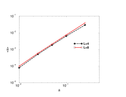
Figure 1: $a$ dependence of the global minima $\langle s\rangle$ of $V_{eff}$. Horizontal axis is lattice spacing $a$, Vertical one is $\langle s\rangle$. We take here $g_{2}=1$, the solid line is for volume $L=8$, while the dashed line is for $L=4$.

.

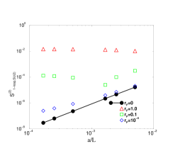
Figure 2: ($1/N$, $\bar{\mu}_{F}=r_{F}/N$) dependence of the nonabelian part of the 1-loop mass correction from the non-zero momentum mode. The horizontal axis is $\frac{1}{N}$ and the vertical axis is $S^{(2)}_{1-loop~{}SU(2)}$.

3.1.2 2-point function

We next study whether the contribution from the non-zero momentum mode integral to the 2-point functions

$$(S^{(2)}_{1-loop})^{\alpha_{1}\alpha_{2}}_{\mu\nu} =[ \delta_{\mu,0}\delta_{\nu,0}+\delta_{\mu,2}\delta_{\nu,2}][2\delta^{\alpha_{1},0}\delta^{\alpha_{2},0}S^{(2)}_{1-loop,~{}U(1)}+2M\delta^{\alpha_{1},\alpha_{2}}S^{(2)}_{1-loop,~{}SU(2)}]$$ (4)

are relevant or not in the continuum limit. The numerical results of $S^{(2)}_{1-loop,~{}SU(2)}$ for several values of ($1/N=a/L$, $\bar{\mu}_{F}\equiv r_{F}/N=a\mu_{F}$) with $\bar{\mu}\equiv a\mu=1/N$ are given in Fig. 2 with $r_{F}$ fixed. $S^{(2)}_{1-loop,~{}U(1)}$ behaves same way as $S^{(2)}_{1-loop,~{}SU(2)}$.

From Fig. 2, we find that the 1-loop correction for $r_{F}\neq 0$ does not vanish in the continuum limit, while that for $r_{F}=0$ vanishes. We should avoid these corrections which are independent from the volume $L$. It becomes clear that one should adopt the following procedure in order to avoid the appearance of such counter terms;

1. Compute physical quantities for fixed ($1/N$, $\bar{\mu}_{F}=r_{F}/N$),

2. Take $\mu_{F}\to 0$ with fixed $1/N$ first , i.e $r_{F}\to 0$,

3. Then take the continuum limit, i.e. $1/N\to 0$ .

This two-step limit can avoid the counter terms as can be seen from Fig. 2 and Eq. (V.17) of Ref.[7] and make any loop correction for effective action irrelevant.

3.2 Zero mode contributions

We now carry out the nonperturbative integral over the zero momentum mode for the 1- and 2-point functions. Since no term of 1-loop contributions from non-zero momentum modes to the effective action can survive in the continuum limit, in order to evaluate 1- and 2-point functions in the continuum limit, we only have to perform the following integral

$$I_{n}^{\alpha_{1}\cdots\alpha_{n}}=L^{\frac{3n}{2}}g_{2}^{\frac{n}{2}}\frac{\int d\tilde{\phi}(\mathbf{0})det[D_{\psi}(\mathbf{0})]\displaystyle{\prod_{i=1}^{n}}(\tilde{s}^{\alpha_{i}}_{\mu}(0))e^{-S_{fin}}}{\int d\tilde{\phi}(\mathbf{0})det[D_{\psi}(\mathbf{0})]e^{-S_{fin}}},$$ (5)

$$S_{fin}=\sum_{\mu>\nu}Tr[\tilde{\phi}_{\mu}(0),\tilde{\phi}_{\nu}(0)]^{2}+\frac{\mu}{g_{2}}Tr[(\tilde{s}_{x}(0)^{2}+\tilde{s}_{y}(0)^{2})].$$ (6)

Among these integral, only the $SU(2)$ part of the 2-point function $I_{2}^{a,b}$ becomes relevant for the discussion whether fine-tuning is needed or not. Since $I_{2}^{a,b}$ is the zero momentum mode of the propagator, it can be written as $I_{2}^{a,b}=\delta^{a,b}L^{2}m_{R}^{-2}$ where $m_{R}^{2}$ is the renormalized mass squared. In order to numerically evaluate the 2-point function $I_{2}^{a,b}=\delta^{a,b}<ss>$, we carry out simulations in the Metropolis algorithm with $2.0\times 10^{5}$ sweeps for the thermalization and $2.0\times 10^{7}$ sweeps for the measurement. We estimate the error by the variance with binsize of $100$ sweeps. Since the 2-point function depends only on the product $g_{2}L$, we take $g_{2}=1$ without loosing generality. Fig. 3 shows the $L$ dependence of the 2-point function.

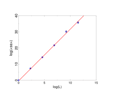
Figure 3: The lattice size $L$ dependence of the 2-point function. The horizontal axis is $L$, where as the vertical axis is $\langle ss\rangle$.

As can be seen in Fig. 3, we find that $\langle ss\rangle$ increases with $L$. Fitting the data with the following function $\langle ss\rangle\sim AL^{3+\alpha}$, we obtain $A=0.65(20)$ and $\alpha=0.210(46)$. This gives the $L$ dependence of the renormalized mass

$$m_{R}2\equiv\frac{\mu^{2}}{g_{2}^{2}}+\Delta\mu^{2}\equiv L^{2}\langle ss\rangle^{-1}\sim\frac{1}{AL^{1+\alpha}},$$ (7)

which vanishes in the large volume limit $L\to\infty$. Our result also implies that the contribution from the quantum corrections becomes dominant for large $L$. Thus in the continuum limit for finite volume, there is a non-trivial mass correction which is larger than the tree level contribution $\frac{\mu}{g_{2}}$. However, after taking the infinite volume limit the mass term vanishes so that there is no need for fine-tuning.

4 Summary and conclusion

We studied the CKKU model  [1] for the supersymmetric U(2) gauge theory in two dimensions structure by an explicit perturbative calculation of scalar one-point and two-point functions. We pointed out that the naive perturbative calculation suffers from the infra-red divergences due to the flat directions in the zero momentum modes of gauge fields and fermion fields [6]. In order to avoid the infra-red divergence for the fermion zero mode, we introduce a new soft susy breaking mass term for the fermion fields. For the bosonic fields, we apply the perturbation only for the non-zero momentum mode and treat the zero momentum mode non-perturbatively. We found that there appears non-trivial quantum mass corrections in the continuum limit. However these corrections vanish in the infinite volume limit so that the CKKU model does not need fine-tuning to recover the full supersymmetry. In addition to the fine-tuning problem discussed in this proceeding, several interesting results are obtained by our explicit calculation as seen in Ref. [7]. Firstly, we found the constraint for the parameter region where the lattice theory is well-defined. And secondly, it is found that the fermion-boson cancellation which suppresses the quantum corrections to the potential is needed to stabilize the deconstructed spacetime in the physical region where the lattice size is larger than the correlation length. Similar instability has been observed in the non-perturbative study [6] on the bosonic part of the CKKU model for the (4,4) 2d super-Yang-Mills [2]. For more details see Ref. [7].

References

- [1] A. G. Cohen, D. B. Kaplan, E. Katz, M. Unsal, JHEP 0308, 024 (2003) [arXiv:hep-lat/0302017].
- [2] D. B. Kaplan, E. Katz, M. Unsal, JHEP 05, 037 (2003) [arXiv:hep-lat/0206019]. A. G. Cohen, D. B. Kaplan, E. Katz, M. Unsal, JHEP 0312, 031 (2003) [arXiv:hep-lat/0307012]. D. B. Kaplan and M. Unsal, [arXiv:hep-lat/0503039].
- [3] S. Catterall and S. Karamov, Nucl. Phys. Proc. Suppl. 106, 935 (2002) [arXiv:hep-lat/0110071]. S. Catterall, JHEP 0305, 038 (2003) [arXiv:hep-lat/0301028]. S. Catterall, S. Karamov, Phys. Rev. D68, 014503 (2003) [arXiv:hep-lat/0305002]. S. Catterall, S. Ghadab, JHEP 0405, 044 (2004) [arXiv:hep-lat/0311042]. S. Catterall, JHEP 0411, 006, (2004) [arXiv:hep-lat/0410052]. S. Catterall, [arXiv:hep-lat/0503036]. F. Sugino, JHEP 0401, 015 (2004) [arXiv:hep-lat/0311021]. F. Sugino, JHEP 0403, 067 (2004) [arXiv:hep-lat/0401017]. F. Sugino, [arXiv:hep-lat/0409036]. F. Sugino, JHEP 0501, 016 (2005) [arXiv: hep-lat/0410035]. A. D’Adda, I. Kanamori, N. Kawamoto and K. Nagata Nucl. Phys. B707, 100 (2005) [arXiv:hep-lat/0406029]. A. D’Adda, I. Kanamori, N. Kawamoto and K. Nagata Nucl. Phys. Proc. Suppl. 140, 754 (2005) [arXiv:hep-lat/0409092]. K. Itoh, M. Kato, H. Sawanaka, H. So and N. Ukita, JHEP 0302, 033 (2003) [arXiv:hep-lat/0210049]. H. Suzuki and Y. Taniguchi, [arXiv:hep-lat/0507019].
- [4] M. R. Douglas, G. W. Moore, [arXiv:hep-th/9603167]. S. Kachru, E. Silverstein, Phys. Rev. Lett. 80, 4855 (1998) [arXiv:hep-th/9802183].
- [5] N. Arkani-Hamed, A. G. Cohen, H. Georgi, Phys. Rev. Lett. 86, 4757 (2001) [arXiv:hep-th/0104005]. N. Arkani-Hamed, A. G. Cohen, D. B. Kaplan, A. Karch, and L. Motl JHEP 0301, 083 (2003) [arXiv:hep-th/0110146].
- [6] J. Giedt, Nucl. Phys. B668, 138 (2003) [arXiv: hep-lat/0304006]. J. Giedt, Nucl. Phys. B674, 259 (2003) [arXiv:hep-lat/0307024]. J. Giedt, [arXiv:hep-lat/0312020]. J. Giedt, [arXiv: hep-lat/0405021].
- [7] T. Onogi and T. Takimi, to be published in Physical Review D. [arXiv:hep-lat/0506014].
- [8] M. Unsal [arXiv: hep-lat/0504016]
- [9] H. Kawai, R. Nakayama, and K. Seo Nucl. Phys. B189, 40 (1981).
- [10] T. Suyama, A. Tsuchiya Prog. Theor. Phys. 99, 321 (1998) [arXiv:hep-th/9711073].