Cho-Faddeev-Niemi decomposition of lattice Yang-Mills theory and evidence of a novel magnetic condensation

Abstract:

We present the first implementation of the Cho–Faddeev–Niemi decomposition of the SU(2) Yang-Mills field on a lattice. Our construction retains the color symmetry (global SU(2) gauge invariance) even after a new type of Maximally Abelian gauge, as explicitly demonstrated by numerical simulations.

PoS(LAT2005)332

1 Introduction

The Cho-Faddeev-Niemi (CFN) decomposition, or a change of variables of the non-Abelian gauge potential in Yang–Mills theory, was proposed by Cho [1] and Faddeev and Niemi [2]. CFN decomposition introduces a color vector field $\mathbf{n}(x)$ enabling us to extract explicitly the magnetic monopole as a topological degree of freedom from the gauge potential without introducing the fundamental scalar field in Yang–Mills theory. The CFN decomposition has been formulated and extensively studied on the continuum spacetime. For non-perturbative studies, however, it is desirable to put the CFN decomposition on a lattice. This will enable us to perform powerful numerical simulations to obtain fully non-perturbative results.

The main purpose of this paper is to propose a lattice formulation of the CFN decomposition and to perform the numerical simulations on the lattice, paying special attention to the magnetic condensations. Our lattice formulation reflects a new viewpoint proposed by three of the authors in a previous paper [4], which enables us to retain the local and global gauge invariance even after the new type of MAG. In the whole of this paper, we restrict the gauge group to SU(2).

2 CFN decomposition in the continuum

We adopt the Cho-Faddeev-Niemi (CFN) decomposition for the non-Abelian gauge field [1, 2, 7]. By introducing a unit vector field $\mathbf{n}(x)$ with three components, i.e., $\mathbf{n}(x)\cdot\mathbf{n}(x):=n^{A}(x)n^{A}(x)=1$ $(A=1,2,3)$, the non-Abelian gauge field $\mathscr{A}_{\mu}(x)$ in the SU(2) Yang-Mills theory is decomposed as

$$\mathscr{A}_{\mu}(x)=c_{\mu}(x)\mathbf{n}(x)+g^{-1}\partial_{\mu}\mathbf{n}(x)\times\mathbf{n}(x)+\mathbb{X}_{\mu}(x).$$ (1)

We use the notation: $\mathbb{C}_{\mu}(x):=c_{\mu}(x)\mathbf{n}(x)$, $\mathbb{B}_{\mu}(x):=g^{-1}\partial_{\mu}\mathbf{n}(x)\times\mathbf{n}(x)$ and $\mathbb{V}_{\mu}(x):=\mathbb{C}_{\mu}(x)+\mathbb{B}_{\mu}(x)$. By definition, $\mathbb{C}_{\mu}(x)$ is parallel to $\mathbf{n}(x)$, while $\mathbb{B}_{\mu}(x)$ is orthogonal to $\mathbf{n}(x)$. We require $\mathbb{X}_{\mu}(x)$ to be orthogonal to $\mathbf{n}(x)$, i.e., $\mathbf{n}(x)\cdot\mathbb{X}_{\mu}(x)=0$. We call $\mathbb{C}_{\mu}(x)$ the restricted potential, while $\mathbb{X}_{\mu}(x)$ is called the gauge-covariant potential and $\mathbb{B}_{\mu}(x)$ is called the non-Abelian magnetic potential. In the naive Abelian projection, $\mathbb{C}_{\mu}(x)$ corresponds to the diagonal component, while $\mathbb{X}_{\mu}(x)$ corresponds to the off-diagonal component, apart from the vanishing magnetic part $\mathbb{B}_{\mu}(x)$.

Accordingly, the non-Abelian field strength $\mathscr{F}_{\mu\nu}(x)$ is decomposed as

$$\mathscr{F}_{\mu\nu}:=\partial_{\mu}\mathscr{A}_{\nu}-\partial_{\nu}\mathscr{A}_{\mu}+g\mathscr{A}_{\mu}\times\mathscr{A}_{\nu}=\mathbb{E}_{\mu\nu}+\mathbb{H}_{\mu\nu}+\hat{D}_{\mu}\mathbb{X}_{\nu}-\hat{D}_{\nu}\mathbb{X}_{\mu}+g\mathbb{X}_{\mu}\times\mathbb{X}_{\nu},$$ (2)

where we have introduced the covariant derivative in the background field $\mathbb{V}_{\mu}$ by $\hat{D}_{\mu}[\mathbb{V}]\equiv\hat{D}_{\mu}:=\partial_{\mu}+g\mathbb{V}_{\mu}\times,$ and defined the two kinds of field strength:

$$\mathbb{E}_{\mu\nu}= E_{\mu\nu}\mathbf{n},\quad E_{\mu\nu}:=\partial_{\mu}c_{\nu}-\partial_{\nu}c_{\mu},$$ (3)

$$\mathbb{H}_{\mu\nu}= H_{\mu\nu}\mathbf{n},H_{\mu\nu}:=-g^{-1}\mathbf{n}\cdot(\partial_{\mu}\mathbf{n}\times\partial_{\nu}\mathbf{n}).$$ (4)

We here notice that $\mathbb{G}_{\mu\nu}:=\mathbb{E}_{\mu\nu}+\mathbb{H}_{\mu\nu}$ is gauge invariant, while each of $\mathbb{E}_{\mu\nu}$ and $\mathbb{H}_{\mu\nu}$ is not gauge invariant. We can define gauge invariant monopole, called CFN monopole, using the field strength $\mathbb{G}_{\mu\nu}$[3].

3 CFN decomposition on a lattice

We discuss how the CFN decomposition is implemented on a lattice by defining the unit color vector field $\mathbf{n}_{x}$ to generate the ensemble of $\mathbf{n}$-fields[3]. On lattice simulation, we can generate the configurations of SU(2) link variables $\{U_{x,\mu}\}$, $U_{x,\mu}=\exp[-ig\epsilon\mathscr{A}_{\mu}(x)],$ using the standard Wilson action, where $\epsilon$ is the lattice spacing and $g$ is the coupling constant. We use the continuum notation for the Lie-algebra valued field variables, e.g., $\mathscr{A}_{\mu}(x)$, even on a lattice. To obtain the configuration with the same Boltzmann weight as the original YM theory, we define CFN decomposition on a lattice based on gauge symmetry of CFN variables.

We define the CFN-Yang–Mills theory as the Yang-Mills theory written in terms of the CFN variables. It has been shown [4] that the SU(2) CFN-Yang–Mills theory has the local gauge symmetry $\tilde{G}_{local}^{\omega,\theta}:=SU(2)_{local}^{\omega}\times[SU(2)/U(1)]_{local}^{\theta}$ larger than one of the original Yang-Mills theory $SU(2)_{local}^{\omega}$, since we can rotate the CFN variable $\mathbf{n}(x)$ by angle $\mathbf{\theta}^{\perp}(x)$ independently of the gauge transformation of $\mathscr{A}_{\mu}(x)$ by the parameter $\mathbf{\omega}(x)$. In order to fix the whole enlarged local gauge symmetry $\tilde{G}_{local}^{\omega,\theta}$, we must impose sufficient number of gauge fixing conditions. Recently, it has been clarified [4] how the CFN-Yang–Mills theory can be equivalent to the original Yang-Mills theory by imposing a new type of gauge fixing called the new Maximal Abelian gauge (nMAG) to fix the extra local gauge invariance in the continuum formulation, see Fig.2.

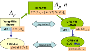
Figure 1: Gauge symmetery of CFN-Yang-Mills theory

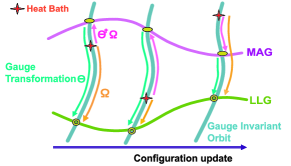
Figure 2: Lattice CFN decomposition obtained by imposing nMAG and LLG

Corresponding to CFN Yang Mills theory in continuum, we define nMAG on a lattice. By introducing a vector field $\mathbf{n}_{x}$ of a unit length with three components, we consider a functional $F_{nMAG}[U,\mathbf{n};\Omega,\Theta]$ written in terms of the gauge (link) variable $U_{x,\mu}$ and the color (site) variable $\mathbf{n}_{x}$ defined by

$$F_{nMAG}[U,\mathbf{n};\Omega,\Theta]:=\sum_{x,\mu}\mathrm{tr}(\mathbf{1}-{}^{\Theta}\mathbf{n}_{x}{}^{\Omega}U_{x,\mu}{}^{\Theta}\mathbf{n}_{x+\mu}{}^{\Omega}U_{x,\mu}^{\dagger}).$$ (5)

Here we have introduced the enlarged gauge transformation: ${}^{\Omega}U_{x,\mu}:=\Omega_{x}U_{x,\mu}\Omega_{x+\mu}^{\dagger}$ for the link variable $U_{x,\mu}$ and ${}^{\Theta}\mathbf{n}_{x}:=\Theta_{x}\mathbf{n}_{x}^{(0)}\Theta_{x}^{\dagger}$ for an initial site variable $\mathbf{n}_{x}^{(0)}$ where gauge group elements $\Omega_{x}$ and $\Theta_{x}$ are independent SU(2) matrices on a site $x$. The former corresponds to the $SU(2)^{\omega}$ gauge transformation $(\mathscr{A}_{\mu})^{\omega}(x)$ of the original potential, while the latter to the adjoint $[SU(2)/U(1)]^{\theta}$ rotation, (see Fig.2).

After imposing the nMAG, the theory still has the local gauge symmetry $SU(2)_{local}^{\omega=\theta}:=SU(2)_{local}^{II}$. Therefore, $\mathbf{n}_{x}$ configuration can not be determined at this stage. In order to completely fix the gauge and determine $\mathbf{n}_{x}$, we need to impose another gauge fixing condition for fixing $SU(2)_{local}^{II}$. In this paper we choose the conventional Lorentz-Landau gauge or Lattice Landau gauge (LLG) for this purpose. The LLG can be imposed by minimizing the function: $F_{LLG}[U;\Omega]=\sum_{x,\mu}\mathrm{tr}(\mathbf{1}-{}^{\Omega}U_{x,\mu})$ with respect to the gauge transformation $\Omega_{x}$, (See Fig. 2). The LLG fixes the local gauge symmetry $SU(2)_{local}^{\omega=\theta}=SU(2)_{local}^{II}$, while the LLG leaves the global symmetry SU(2)${}_{global}^{\omega}=SU(2)_{global}^{II}$ intact. Therefore, we define the lattice nMAG by minimizing the functional $F_{nMAG}[U,\mathbf{n};\Omega,\Theta]$ with respect to the gauge transformation $\{\Omega_{x}\}$ and $\{\Theta_{x}\}$, and we obtain the lattice CFN decomposition:

$${}^{\Omega}U_{x,\mu}=\exp\{-i\epsilon g[\mathbb{C}_{\mu}(x)+\mathbb{B}_{\mu}(x)+\mathbb{X}_{\mu}(x)]\}.$$ (6)

Then a remaining issue to be clarified is how to construct the ensemble of the color $\mathbf{n}$-fields used in defining $F_{nMAG}[U,\mathbf{n};\Omega,\Theta]$ and $U_{x,\mu}$. Now it is shown that the desired color vector field $\mathbf{n}_{x}$ is constructed from the interpolating gauge transformation matrix $\Theta_{x}$ according to $\mathbf{n}_{x}^{(0)}=\sigma_{3}$ and

$$\mathbf{n}_{x}:=\Theta_{x}\sigma_{3}\Theta_{x}^{\dagger}=n_{x}^{A}\sigma^{A},\quad n_{x}^{A}=\mathrm{tr}[\sigma_{A}\Theta_{x}\sigma_{3}\Theta_{x}^{\dagger}]/2\quad(A=1,2,3).$$ (7)

The first observation is that the functional $F_{nMAG}[U,\mathbf{n};\Omega,\Theta]$ has another equivalent form $F_{nMAG}[U,\mathbf{n};\Omega,\Theta]=F_{MAG}[U;G]=\sum_{x,\mu}\mathrm{tr}(\mathbf{1}-\sigma_{3}\ {}^{G}{}U_{x,\mu}\ \sigma_{3}\ {}^{G}{}U_{x,\mu}^{\dagger})$, with the identification $G_{x}:=\Theta_{x}^{\dagger}\Omega_{x}$. This procedure determines the configurations $\{G_{x}^{\ast}\}$ of SU(2) variables achieving the minimum of $F_{MAG}[U;G],$ (See Fig. 2).

On a gauge orbit, two representatives on the two gauge-fixing hypersurfaces (MAG and LLG) are connected by the gauge transformation $\Theta\equiv\Omega^{\ast}(G^{\ast})^{\dagger}$. Thus we can determine a set of interpolating gauge-rotation matrices $\{\Theta_{x}\}$ to construct $\mathbf{n}_{x}$ ensemble. In fact, the color vector $\mathbf{n}_{x}$ constructed in this way represents a real-valued vector $\vec{n}_{x}=(n_{x}^{1},n_{x}^{2},n_{x}^{3})$ of unit length with three components, and transforms in the adjoint representation under the gauge transformation II.

By imposing simultaneously the nMAG and the LLG in this way, we can completely fix the whole local gauge invariance $\tilde{G}_{local}^{\omega,\theta}$ of the lattice CFN-Yang–Mills theory. It should be remarked that, even after the gauge fixing, the global (color) symmetry $SU(2)_{global}^{\omega=\theta}$ is unbroken.

Finally, we give the explicit expressions of CFN variables on lattice, from link variable $U$ and $\mathbf{n}$-fields. In the continuum theory, the CFN decomposition is uniquely obtained as $c_{\mu}(x)=\mathbf{n}(x)\mathbf{\cdot}\mathscr{A}_{\mu}(x)$ and $\mathbb{X}_{\mu}=g^{-1}\mathbf{n}(x)\mathbf{\times}\hat{D}_{\mu}[\mathscr{A}_{\mu}]\mathbf{n}(x)$ for the given gauge potential $\ \mathscr{A}_{\mu}(x)$ and $\mathbf{n}$-field [6].  Thus CFN variables on a lattice can be defined by the gauge potential $g\epsilon\mathbb{A}_{x,\mu}:=\frac{i}{2}\left(U_{x,\mu}-U_{x,\mu}^{\dagger}\right),$ using U-linear definition. We define the differential of $n$-field as a forwarded differential corresponding to a link variable, $\Delta_{\mu}\vec{n}(x):=\vec{n}(x+\epsilon\hat{\mu})-\gamma_{\mu}(x)\vec{n}(x)$, where $\hat{\mu}$ is a unit vector to the direction $\mu$. The coefficient $\gamma_{\mu}(x)=\vec{n}(x+\epsilon\hat{\mu})\cdot\vec{n}(x)$ is defined to satisfy the orthogonal condition $\Delta_{\mu}\vec{n}(x)\cdot\vec{n}(x)=0$ ($\partial_{\mu}\vec{n}(x)\cdot\vec{n}(x)=0$ in continuum theory). So the CFN variables on a lattice are obtained as follows;

$$\qquad\mathbb{B}_{x,\mu} :=\Delta_{\mu}\vec{n}_{x}\times\vec{n}_{x}=\vec{n}_{x+\epsilon\hat{\mu}}\times\vec{n}_{x},$$ (8)

$$c_{x,\mu} =\mathbb{A}_{x,\mu}\cdot\mathbf{n}_{x},\qquad\mathbb{X}_{x,\mu}:=\mathbb{A}_{x,\mu}-c_{x,\mu}\mathbf{n}_{x}-\mathbb{B}_{x,\mu}.$$ (9)

4 Numerical simulations

Our numerical simulations are performed as follows. In the continuum formulation, the CFN variables were introduced as a change of variables in such a way that they do not break the global gauge symmetry $SU(2)_{global}^{II}$ or ”color symmetry”, corresponding to the global gauge symmetry $SU(2)_{global}^{I}$ in the original Yang-Mills theory. Hence the nMAG can be imposed in terms of the CFN variables without breaking the color symmetry. This is a crucial difference between the nMAG based on the CFN decomposition and the conventional MAG based on the ordinary Cartan decomposition which breaks the $SU(2)_{global}$ explicitly. Therefore, we must perform the numerical simulations so as to preserve the color symmetry as much as possible. This is in fact possible as follows.

Remember that the nMAG on a lattice is achieved by repeatedly performing the gauge transformations. In order to preserve the global SU(2) symmetry, we adopt a random (global) gauge transformation only in the first sweep among the whole sweeps of gauge transformations in the standard iterative gauge fixing procedure for the LLG. This procedure moves an ensemble of unit vectors $\mathbf{n}_{x}$ to a random ensemble of $\mathbf{n}_{x}$ which is far away from $\mathbf{n}_{x}=(0,0,1)$. Then we search for the local minima around this configuration of $\mathbf{n}_{x}$ by performing the successive gauge transformations. The first random gauge transformation as well as the subsequent gauge transformations are accumulated to obtain the gauge transformation matrix $\Theta$ by which $\mathbf{n}$ is constructed.

4.1 Lattice data

Our numerical simulations are performed on the lattice with the lattice size $L^{4}=$ $24^{4}$ by using heat-bath method for the standard Wilson action[8] for the gauge coupling $\beta=2.3\sim 2.7$ and periodic boundary conditions. Staring with cold initial condition and thermalizing 50*100 sweeps, we have obtained 200 configurations at intervals of 100 sweeps. For LLG and MAG, we have used the over relaxation algorithm.

We first focus on the $\mathbf{n}$-fields. We have measured expectation values $\left\langle n_{x}^{A}\right\rangle$ $(A=1,2,3)$, and have obtained the vanishing expectation values. Moreover, we have measured the two-point correlation functions defined by $\left\langle n_{x}^{A}n_{0}^{B}\right\rangle$, see Fig. 4. The two-point correlation functions $\left\langle n_{x}^{A}n_{0}^{A}\right\rangle$ (no summation over $A$) exhibit almost the same behavior in all the directions ($A=1,2,3$), while $\left\langle n_{x}^{A}n_{0}^{B}\right\rangle$ ($A\not=B$) vanish. Thus, we have obtained the correlation function $\left\langle n_{x}^{A}n_{0}^{B}\right\rangle=\delta^{AB}D(x)$ respecting color symmetry. These results indicate that the global $SU(2)$ symmetry (color symmetry) is unbroken in our main simulations.

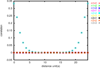
Figure 3: ¡nn¿ correlation

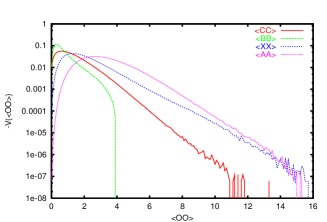
Figure 4: constraint effective potential

Secondary, we focus on the anatomy of the condensation by CFN variables. We measure the ”naive” condensation of mass dimension 2; $\left(g\epsilon\right)^{2}\left\langle\mathbb{A}_{x,\mu}^{2}\right\rangle=\left(g\epsilon\right)^{2}\left[\left\langle c_{x,\mu}^{2}\right\rangle+\left\langle\mathbb{B}_{x,\mu}^{2}\right\rangle+\left\langle\mathbb{X}_{x,\mu}^{2}\right\rangle+2\left\langle\mathbb{B}_{x,\mu}\mathbb{X}_{x,\mu}\right\rangle\right]$, and have obtained the non-zero value of condensaions of CFN variables. We also measure the ”constraint effective potential” defined by probability distribution of a local operator $\Phi(x);$ Pr$(\phi)=\left\langle\delta\left(\phi(x)-\Phi(x)\right)\right\rangle$ and the effective potential is defined by $V_{eff}(\phi)=-\ln\left\langle\delta\left(\phi(x)-\Phi(x)\right)\right\rangle.$ Here, we measure effective potential for $\Phi(x)=\left\{\mathbb{A}_{x,\mu}^{2},\text{ }c_{x,\mu}^{2},\text{ }\mathbb{B}_{x,\mu}^{2},\text{ }\mathbb{X}_{x,\mu}^{2},...\right\}$. Fig. 4 shows that effective potential $-V_{eff}(\phi)$ has peaks at nonzero expectation value $\left\langle\Phi(x)\right\rangle.$ This suggest that we can expect non-zero condensations.

5 Summary and Discussion

We have shown how to implement the CFN decomposition (change of variables) of SU(2) Yang–Mills theory on a lattice, according to a new viewpoint proposed in [4]. A remarkable point is that our approach can preserve both the local SU(2) gauge symmetry and the color symmetry (global SU(2) symmetry) even after imposing a new type of gauge fixing (called the nMAG) which is regarded as a constraint to reproduce the original Yang-Mills theory.

Moreover, we have succeeded to perform the numerical simulations in such a way that the color symmetry is unbroken. This is the first remarkable result. This is in sharp contrast to the previous approaches [10, 9]. Although the similar technique of constructing the unit vector field $\mathbf{n}_{x}$ from a $SU(2)$ matrix $\Theta$ has already appeared, e.g., in [10, 9, 11], there is a crucial conceptual difference between our approach and others.

We have shown preliminary result for the anatomy of the condensation of mass dimension 2. We have obtained the result suggesting non-zero value of the condensations. To determine the physical value of the condensation, we need the further study such as the renomalization of the CFN variables.

References

- [1] Y.M. Cho, Phys. Rev. D 21, 1080 (1980). Phys. Rev. D 23, 2415 (1981).
- [2] L. Faddeev and A.J. Niemi, [hep-th/9807069], Phys. Rev. Lett. 82, 1624 (1999).
- [3] S. Kato, K.-I. Kondo, T. Murakami, A. Shibata and T. Shinohara, and S. Ito, hep-lat/0509069
- [4] K.-I. Kondo, T. Murakami and T. Shinohara, hep-th/0504107.
- [5] K.-I. Kondo, [hep-th/0404252], Phys.Lett. B 600, 287 (2004).
- [6] S. Kato, K.-I. Kondo, T. Murakami, A. Shibata and T. Shinohara, hep-ph/0504054.
-
[7]
S.V. Shabanov,
[hep-th/9903223], Phys. Lett. B 458, 322
(1999).
S.V. Shabanov, [hep-th/9907182], Phys. Lett. B 463, 263 (1999). - [8] M. Creutz, Phys. Rev. D21, 2308 (1980).
- [9] S.V. Shabanov, [hep-lat/0110065], Phys. Lett. B 522, 201 (2001).
- [10] L. Dittmann, T. Heinzl and A. Wipf, [hep-lat/0210021], JHEP0212, 014 (2002).
- [11] H. Ichie and H. Suganuma, [hep-lat/9808054], Nucl. Phys. B 574, 70 (2000).