Pionic couplings $\widehat{g}$ and $\widetilde{g}$
in the static heavy quark limit

Abstract:

The couplings between the soft pion and the doublet of heavy-light mesons are basic parameters of the ChPT approach to the heavy-light systems. We compute the unquenched ($N_{f}=2$) values of such couplings in the static heavy quark limit: (1) $\widehat{g}$, coupling to the lowest doublet of heavy-light mesons, and (2) $\widetilde{g}$, coupling to the first orbital excitations. A brief description of the calculation together with the short discussion of the results is presented.

PoS(LAT2005)212

1 Physics Motivation

Static quark limit of QCD offers a simplified framework to solving the non-perturbative dynamics of light degrees of freedom, which is highly important for various phenomenological studies of weak interactions involving the heavy-light mesons. In the exact $m_{Q}\to\infty$ limit, the heavy quark symmetry (HQS) constrains the QCD dynamics of light quarks and soft gluons in the heavy-light hadrons to be invariant under the change of the heavy quark flavour and/or its spin ($j_{Q}$). As a result the total angular momentum of the light degrees of freedom becomes a good quantum number ($j_{\ell}^{P}$), and therefore the physical heavy-light mesons come in mass-degenerate doublets:

$$\underbrace{[D(0^{-}),D^{\ast}(1^{-})]}_{j_{\ell}^{P}=\frac{1}{2}^{-}(L=0)}\,,\quad\underbrace{[D_{0}^{\ast}(0^{+}),D_{1}^{\prime}(1^{+})]}_{j_{\ell}^{P}=\frac{1}{2}^{+}(L=1)}\,,\quad\underbrace{[D_{1}(1^{+}),D_{2}^{\ast}(2^{+})]}_{j_{\ell}^{P}=\frac{3}{2}^{+}(L=1)}\,,\quad\dots$$ (1)

where on the example of charmed states we remind the reader of spectroscopic labels. HQS is a basis for the systematic expansion of the QCD Green functions in power series of $\Lambda_{\rm QCD}/m_{Q}$, known as the heavy quark effective theory (HQET). At each order, one has to solve the non-perturbative QCD dynamics of the light degrees of freedom which can actually be done only by the numerical QCD simulations on the lattice.

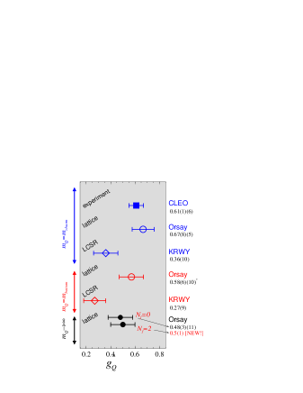
Figure 1: Results for $\widehat{g}$ with the heavy quark being static, bottom or charm. Asterisk on the lattice result for $\widehat{g}_{b}$ indicates that the result is not obtained after interrpolating between the static and charm heavy quark cases. The numbers are taken from refs. [2, 3, 4, 5], in descending order.

Due to inability to simulate directly the dynamics of light quarks that are close enough in mass to the physical $u$- or $d$-quark, one has to make various chiral extrapolations, which induce large systematic errors to the lattice results (a typical example is the one of $SU(3)$ flavour breaking ratio of the pseudoscalar meson decay constants, $f_{B_{s}}/f_{B_{d}}$). In addition the insufficient size of the lattice box with the periodic boundary conditions afflicts the propagation of the light pions on the lattice. To have a good handle on these two problems one can rely on the effective theory that describes the dynamics of light degrees of freedom in terms of pseudo-Goldstone bosons (pions,, for short), usually referred to as heavy meson chiral perturbation theory (HMChPT) [1]. HMChPT is suitable when working with (nearly) massless quarks and thus it is complementary to the light quark dynamics that is directly accessible from the lattice. Similar to the standard ChPT, where the pion axial coupling ($f_{\pi}$) is a parameter of the theory, in the HQChPT Lagrangians the axial couplings of a pion to doublets of heavy-light mesons are parameters of the theory. In other words, they have to be fixed elsewhere. The most well-known such a coupling is the one with the $(1/2)^{-}$-doublet, known as $\widehat{g}$, whose value was experimentally established in the case of heavy charm quark [2]. That value appeared to be much larger than the ones predicted by most of the relativistic quark models and by all the QCD sum rules. In fig. 1, we show the panorama of the results for that coupling obtained by using lattices and light cone QCD sum rules (LCSR). Lattice values are obtained both in the static heavy quark limit [5, 6] and with the heavy quark of the mass around the physical charm quark mass [3]. However, all the lattice computations of that coupling are obtained in the quenched approximation. In this note, we present the first unquenched result for $\widehat{g}$, with $N_{f}=2$ dynamical light quarks and in the static heavy quark limit (indicated as ”New” in fig. 1. In addition, we report the first result for $\widetilde{g}$, the coupling of the soft pion to the $(1/2)^{+}$-doublet of heavy-light mesons.

2 Definitions and Correlation functions to be computed

In the limit in which the heavy quark is infinitely heavy and the light quarks are massless, the axial couplings of the charged pion to the heavy-light mesons, $\widehat{g}$ and $\widetilde{g}$, are defined via

$$\langle H|\vec{\cal A}|H^{\ast}(\varepsilon)\rangle=\widehat{g}\ \vec{\varepsilon}\,,\qquad\langle H^{\ast}_{0}|\vec{\cal A}|H^{\prime}_{1}(\varepsilon)\rangle=\widetilde{g}\ \vec{\varepsilon}\,,$$ (2)

where the non-relativistic normalisation of states $|H^{(\ast,\prime)}_{0,1}\rangle$ is assumed, $\langle H_{i}(v)|H_{j}(v^{\prime})\rangle=\delta_{ij}\delta(v-v^{\prime})$. All heavy-light hadrons are at rest ($\vec{v}=\vec{v}^{\prime}=\vec{0}$), and therefore the soft pion which couples to the axial current, ${\cal A}_{\mu}=\bar{u}\gamma_{\mu}\gamma_{5}d$, is also at rest, $\vec{q}=\vec{0}$. $\varepsilon_{\mu}$ is the polarisation of the vector and the axial heavy-light meson respectively.

The standard strategy to compute the above matrix elements consists in evaluating the following two- and three- point correlation functions:

$$C_{2}(t) = \langle\sum_{\vec{x}}P(x)P^{\dagger}(0)\rangle_{{}_{U}}=\frac{1}{3}\langle\sum_{i,\vec{x}}V_{i}(x)V_{i}^{\dagger}(0)\rangle_{{}_{U}}=\langle\sum_{\vec{x}}{\rm Tr}\left[{1+\gamma_{0}\over 2}P_{x}^{0}\gamma_{5}{\cal S}_{u,d}(0,x)\gamma_{5}\right]\rangle_{{}_{U}},$$

$$\widetilde{C}_{2}(t) = \langle\sum_{\vec{x}}S(x)S^{\dagger}(0)\rangle_{{}_{U}}=\frac{1}{3}\langle\sum_{i,\vec{x}}A_{i}(x)A_{i}^{\dagger}(0)\rangle_{{}_{U}}=\langle\sum_{\vec{x}}{\rm Tr}\left[{1+\gamma_{0}\over 2}P_{x}^{0}{\cal S}_{u,d}(0,x)\right]\rangle_{{}_{U}},$$

$$C_{3}(t_{x}) = \langle\sum_{\vec{x},\vec{y}}P(y){\cal A}_{i}(x)V_{i}^{\dagger}(0)\rangle=\langle\sum_{\vec{x},\vec{y}}{\rm Tr}\left[{1+\gamma_{0}\over 2}P_{y}^{0}\gamma_{i}{\cal S}_{u}(0,x)\gamma_{i}\gamma_{5}{\cal S}_{d}(x,y)\gamma_{5}\right]\rangle_{{}_{U}},$$ (3)

$$\widetilde{C}_{3}(t_{x}) = \langle\sum_{\vec{x},\vec{y}}S(y){\cal A}_{i}(x)A_{i}^{\dagger}(0)\rangle_{{}_{U}}=\langle\sum_{\vec{x},\vec{y}}{\rm Tr}\left[{1+\gamma_{0}\over 2}P_{y}^{0}\gamma_{i}\gamma_{5}{\cal S}_{u}(0,x)\gamma_{i}\gamma_{5}{\cal S}_{d}(x,y)\right]\rangle_{{}_{U}},$$

where $\langle\dots\rangle_{{}_{U}}$ denotes the average over independent gauge field configurations. The gauge field configurations used in this work are the ones produced by the SPQcdR collaboration [7]. The interpolating fields that we use to produce the desired $(1/2)^{\mp}$ heavy-light mesons are: $P=\bar{h}\gamma_{5}q$, $V_{i}=\bar{h}\gamma_{i}q$, $S=\bar{h}q$, and $A_{i}=\bar{h}\gamma_{i}\gamma_{5}q$, with $q$ being either $u$- or $d$-quark field. In eq. (2) we also express the correlation functions in terms of quark propagators: light ones, ${\cal S}_{u,d}(0,x)$, and the infinitely heavy one (the Wilson line),

$$P_{x}^{0}=\delta(\vec{x})\prod_{\tau=0}^{t_{x}-1}U_{0}(\tau)\,,$$ (4)

where $U_{0}$ is the temporal component of the link variable. The spectral decomposition of the three point function $C_{3}(t_{x})$ reads

$$C_{3}(t_{x})=\sum_{m,n}\Big{[}\underbrace{\langle 0|P|H_{n}\rangle}_{Z_{n}}e^{-E_{H_{n}}t_{y}}\langle H_{n}|{\cal A}_{i}|H^{\ast}_{m}\rangle e^{-(E_{H_{m}^{\ast}}-E_{H_{n}})t_{x}}\underbrace{\langle H^{\ast}_{m}|V_{i}|0\rangle}_{Z_{m}\varepsilon_{i}(m)}\Big{]}\,,$$ (5)

with the sum running over the ground states ($m=n=0$) and the radial excitations ($m,n>0$) which are heavier and thus exponentially suppressed. If only the diagonal terms were different from zero [i.e., the terms in the sum (5) with $m=n$], then the function $C_{3}(t_{x})$ would be $t_{x}$-independent because the HQS ensures that $E_{H_{n}^{\ast}}=E_{H_{n}}$. This is indeed what one observes from the lattice data: even for very small values of $t_{x}$ the correlation functions $C_{3}(t_{x})$ and $\widetilde{C}_{3}(t_{x})$ exhibit plateaus (c.f. fig. 2). However, even after leaving out the non-diagonal terms ($m\neq n$), we still have a problem of contamination by the radial excitations ($m=n>0$) in eq. (5). The latter are taken care of by implementing the smearing procedure which highly enhances the overlap of the interpolating fields with the lowest energy states. Once that is been done, it is then trivial to extract the couplings $\widehat{g}$ and $\widetilde{g}$, namely

$${C_{3}(t_{x})\over(Z_{0}^{\rm sm.})^{2}e^{-E_{0}t_{y}}}\longrightarrow\widehat{g}(m_{\pi}^{2})\,,\qquad{\widetilde{C}_{3}(t_{x})\over(\widetilde{Z}_{0}^{\rm sm.})^{2}e^{-\widetilde{E}_{0}t_{y}}}\longrightarrow\widetilde{g}(m_{\pi}^{2})\,.$$ (6)

where $(Z_{0}^{\rm sm.})^{2}$ is extracted from the fit to $C_{2}(t)=\displaystyle{\sum_{n}}|Z_{n}^{\rm sm.}|^{2}\exp(-E_{n}t)$, with smeared sources. Likewise $(\widetilde{Z}_{0}^{\rm sm.})^{2}$ is extracted from $\widetilde{C}_{2}(t)$. Before going to the results, we should stress again that the above identification with the couplings $\widehat{g}$ and $\widetilde{g}$ is valid only in the chiral limit, $g=\displaystyle{\lim_{m_{\pi}^{2}\to 0}g(m_{\pi}^{2})}$.

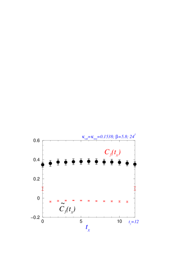
Figure 2: Correlation functions $C_{3}(t_{x})$ and $\widetilde{C}_{3}(t_{x})$ in which the sources are fixed at $0$ and $t_{y}=12$.

3 Lattice details and results

Our dataset consists of $50$ gauge field configurations which include $N_{f}=2$ dynamical quarks whose masses, with respect to the physical strange quark mass, are within the range $0.7\lesssim m_{q}/m_{s}^{phys}\lesssim 1.3$. We use the (unimproved) Wilson quarks and work on $24^{3}\times 48$ lattices at $\beta=5.8$, which corresponds to the lattice spacing of $a\approx 0.06$ fm, and the physical volume $(1.5~{}{\rm fm})^{3}$. The corresponding ”sea” quark hopping parameters ($\kappa_{\rm sea}$) are listed in table 1. More information about the simulations can be found in ref. [7]. In all our computations we keep the valence and sea light quarks equal.

In the computation we used the Eichten–Hill static quark action [8], supplemented by the hypercubic blocking procedure (HYP) of ref. [9] which is known to substantially improve the signal/noise ratio in the correlation functions (2). In that way we were able to monitor the the efficiency of the smearing, i.e., by confronting the signal of $C_{2}(t)$ by using both local sources with the signal in which both sources are being smeared. The generic local source operator is smeared as in ref. [10], $\bar{h}(x)\Gamma q(x)\to\bar{h}(x)\Gamma q^{S}(x)$ where,

$$q^{S}(x)=\sum\limits_{r=0}^{R_{\rm max}}{\scriptstyle(r+\frac{1}{2})}^{2}e^{-r/R}\sum\limits_{k=x,y,z}\left[q({\scriptstyle x+r\hat{k}})\times\prod\limits_{i=1}^{r}U^{F}_{k}({\scriptstyle x+(i-1)\hat{k}})+q({\scriptstyle x-r\hat{k}})\times\prod\limits_{i=1}^{r}U_{k}^{F^{\dagger}}({\scriptstyle x-i\hat{k}})\right]\,,$$ (7)

$U^{F}$ being the so called fuzzed link variable. The parameters $R=3$ and $R_{\rm max}=5$ are tuned to enhance the overlap with the lowest lying state, which we were able to check from the analysis of the two point functions $C_{2}(t)$ and $\widetilde{C}_{2}(t)$. We obtain that $Z_{0}^{\rm sm.}/Z_{0}^{\rm loc.}\approx 150$, while $Z_{1}^{\rm sm.}/Z_{1}^{\rm loc.}<0.05$. Similar situation holds for the scalar-scalar correlation function, and it is therefore safe to say that the pollution of our results for $\widehat{g}(m_{\pi}^{2})$ and $\widetilde{g}(m_{\pi}^{2})$ that comes from the transitions among higher excitations is to a huge extent suppressed by the smearing procedure.

$\kappa_{\rm sea}=\kappa_{\rm val}$	$r_{0}m_{\pi}$	$r_{0}(\widetilde{E}_{0}-E_{0})$	$\widehat{g}(m_{\pi}^{2})$	$\widetilde{g}(m_{\pi}^{2})$
l j $0.1535$	$1.97(5)$	$1.49(11)$	$0.55(4)$	$-0.18(1)$
l j $0.1538$	$1.82(4)$	$1.71(12)$	$0.48(3)$	$-0.20(4)$
l j $0.1540$	$1.72(5)$	$1.60(12)$	$0.52(6)$	$-0.21(4)$
l j $0.1541$	$1.47(7)$	$1.74(19)$	$0.43(4)$	$-0.14(2)$

Table 1: Results for the orbital splitting $\widetilde{E}_{0}-E_{0}$, the couplings $\widehat{g}$ and $\widetilde{g}$, from the unquenched $N_{f}=2$ simulations in which the dynamical quark is of the mass corresponding to the pion whose masses are also given.

Our results for $\widehat{g}(m_{\pi}^{2})$ and $\widetilde{g}(m_{\pi}^{2})$ are given in table 1, and plotted in fig. 3. These results are obtained by fixing one of the source operators to $t_{y}=12$. The stability of these values is checked by using $t_{y}=11$, and $t_{y}=13$. In the same table we also give the mass difference between the lowest lying states belonging to $(1/2)^{+}$ and $(1/2)^{-}$ doublets.

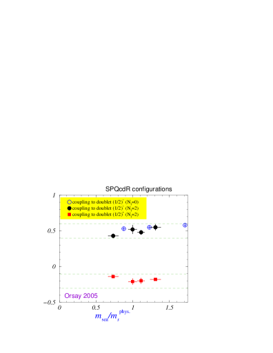
Figure 3: Our new (unquenched) results against the old (quenched) ones. The dashed lines correspond to the range of values that $\widehat{g}(0)$ and $\widetilde{g}(0)$ can assume after the chiral extrapolation.

On the basis of our results, we make the following observations:

• The values of $\widehat{g}(m_{\pi}^{2})$ from the unquenched simulations are consistent with the quenched values we reported in ref. [5] (see also fig. 3);

• The values of $\widetilde{g}(m_{\pi}^{2})$ are clearly negative and their absolute values much smaller than those of $\widehat{g}(m_{\pi}^{2})$;

• The statistical and systematic quality of our data is not good enough to discuss the subtleties of chiral extrapolations. Instead, we quote $0.4\leq\widehat{g}\leq 0.6$, and $-0.3\leq\widetilde{g}\leq-0.1$, as our current estimates;

• Less prone to statistical noise is the ratio $\widetilde{g}/\widehat{g}$, for which we obtain

  $$\widetilde{g}/\widehat{g}=-0.34(3),-0.43(9),-0.39(7),-0.31(6),$$ (8)

  in the order of decreasing light quark mass;

• Our results are in a clear conflict with the assumption, $\widetilde{g}=\widehat{g}$, that stems from the parity doubling models [11];

• Our values of the orbital splitting $\widetilde{E}_{0}-E_{0}$, together with the couplings $\widehat{g}$ and $\widetilde{g}$ do not help to explain the puzzling experimental phenomenon that $(\widetilde{E}_{0}-E_{0})_{s}<(\widetilde{E}_{0}-E_{0})_{u,d}$ [12]. To address this question more seriously it is essential to reduce the sea quark masses, work on larger lattice volumes and increase the statistical quality of our data.

References

• [1] R. Casalbuoni, A. Deandrea, N. Di Bartolomeo, R. Gatto, F. Feruglio and G. Nardulli, Phys. Rept.  281 (1997) 145 [hep-ph/9605342].
• [2] A. Anastassov et al. [CLEO Collaboration], Phys. Rev. D 65 (2002) 032003 [hep-ex/0108043].
• [3] A. Abada et al., Phys. Rev. D 66 (2002) 074504 [hep-ph/0206237]; Nucl. Phys. Proc. Suppl.  119 (2003) 641 [hep-lat/0209092].
• [4] A. Khodjamirian et al., Phys. Lett. B 457 (1999) 245 [hep-ph/9903421], see also P. Ball and R. Zwicky Phys. Rev. D 71 (2005) 014015 [hep-ph/0406232].
• [5] A. Abada et al., JHEP 0402 (2004) 016 [hep-lat/0310050].
• [6] G. M. de Divitiis et al. [UKQCD Collaboration], JHEP 9810 (1998) 010 [hep-lat/9807032].
• [7] D. Becirevic et al., hep-lat/0509091, and hep-lat/0510014.
• [8] E. Eichten and B. Hill, Phys. Lett. B 234 (1990) 511.
• [9] A. Hasenfratz and F. Knechtli, Phys. Rev. D 64 (2001) 034504 [hep-lat/0103029].
• [10] P. Boyle [UKQCD Collaboration], J. Comput. Phys.  179 (2002) 349 [hep-lat/9903033].
• [11] W. A. Bardeen, E. J. Eichten and C. T. Hill, Phys. Rev. D 68 (2003) 054024 [hep-ph/0305049]; M. A. Nowak, M. Rho and I. Zahed, Acta Phys. Polon. B 35 (2004) 2377 [hep-ph/0307102].
• [12] T. Mehen and R. P. Springer, Phys. Rev. D 72 (2005) 034006 [hep-ph/0503134]; D. Becirevic, S. Fajfer and S. Prelovsek, Phys. Lett. B 599 (2004) 55 [hep-ph/0406296].