Algorithm Shootout: R versus RHMC

Abstract:

We present initial results comparing the RHMC and R algorithms on large lattices with small quark masses using chiral fermions. We also present results concerning staggered fermions near the deconfinement/chiral phase transition. We find that the RHMC algorithm not only eliminates the step-size error of the R algorithm, but is also considerably more efficient. We discuss several possibilities for further improvement to the RHMC algorithm.

PoS(LAT2005)115

1 Introduction and Motivation

We start with an observable $\Omega$ measured in the vacuum, $\langle\Omega\rangle=\int{\mathcal{D}}Ue^{-S(U)}[\mathop{\rm det}{\cal M}(U)]^{\alpha}\Omega(U)/Z$, where the parameter $\alpha$ defines the number of fermion flavours the theory represents ($\alpha=N_{f}/4$ for staggered and $N_{f}/2$ for Wilson). We choose to include the operator ${\cal M}=M^{\dagger}M$ as opposed to just $M$ (the Dirac operator) to allow us to update the pseudofermion fields using a heatbath. When $\alpha$ is non-integer, the conventional HMC algorithm fails, and this necessitates another algorithm choice if we are to include the effects due to the strange quark (or even if we want to simulate a two flavour staggered fermion theory).

The most popular algorithm to date for performing such calculations has been the R algorithm (R) [1]. Here the fermionic determinant is rewritten in exponential-trace-logarithm form $\mathop{\rm det}{\cal M}^{\alpha}=\mathop{\rm exp}\left(\alpha\mathop{\rm tr}\mathop{\rm ln}{\cal M}\right)$. When the equations of motion for this effective action are derived, it is found that the explicit matrix inverse is required. To circumvent this problem the trace is replaced by a noisy estimator, this results in a fermionic force term almost identical to that obtained from HMC where a pseudofermion formulation is used. The key difference is that in the former the force is merely a noisy estimator of the true fermion force, whereas in the latter the derived force is exactly the pseudofermion force. This means that the $O(\delta\tau)$ error term in the conserved Hamiltonian no longer cancels automatically, and to force this cancellation an irreversible and non-area preserving integrator must be used. Thus the algorithm cannot be made exact through the inclusion of a Monte Carlo acceptance test and any results generated using R will have finite $O(\delta\tau^{2})$ errors.

2 Rational Hybrid Monte Carlo

The Rational Hybrid Monte Carlo Algorithm (RHMC) was designed to overcome the shortcomings of R, namely the inexact nature of the calculations (for a proper description of the algorithm see [2], the description given here is sparse on details). The fermion determinant is rewritten in pseudofermion formulation, and a rational approximation is used to represent the effective matrix appearing in the bilinear term, $\mathop{\rm det}{\cal M}^{\alpha}=\int{\mathcal{D}}\bar{\phi}{\mathcal{D}}\phi e^{-\bar{\phi}{\cal M}^{-\alpha}\phi}\approx\int{\mathcal{D}}\bar{\phi}{\mathcal{D}}\phi e^{-\bar{\phi}r^{2}({\cal M})\phi}$, with $r(x)\approx x^{-\alpha/2}$ . If the error $\Delta$ on the rational approximation is made arbitrarily small, e.g., $\Delta(x)=\left|1-x^{\alpha/2}r(x)\right|<10^{-14}$, then there can be no systematic bias induced from using a rational approximation and the conventional HMC algorithm can be used, but with the rational function used as the kernel in the bilinear.

Any rational function can be written as a sum of partial fractions, $r(x)=\sum_{k=1}^{n}\alpha_{k}/(x+\beta_{k})$, in this form a multi-shift solver can be used to evaluate all shifts for approximately the same cost as the smallest shift (which is near zero). A lower degree approximation can be used for the MD evolution since any errors are corrected for stochastically when the accept/reject test is performed. This approximation is generally set to $\bar{r}\approx{\cal M}^{-\alpha}\approx r^{2}$ to avoid the double inversion which would have arisen from using $r^{2}$. The resulting pseudofermion force is written

$$S_{\mbox{\tiny F}}^{\prime}=-\sum_{i=1}^{\bar{n}}\bar{\alpha}_{i}\phi^{\dagger}({\cal M}+\bar{\beta}_{i})^{-1}{\cal M}^{\prime}({\cal M}+\bar{\beta}_{i})^{-1}\phi.$$ (1)

Hence the cost of the algorithm is similar to HMC in that it only requires one conjugate gradient inversion per MD step.

3 Finite temperature QCD

The comparison of the algorithms’ performance near the chiral transition point is of particular relevance. In this regime it has been shown that the exact location of the transition point $\beta_{c}$ can be strongly affected by finite step-size errors [3]. The aim of our study was to see how RHMC behaves in this regime, and to compare the cost against using R. The parameters we used are given in Table 2. In Figures 2 and 2 plots of the variation of the plaquette and of $\bar{\psi}\psi$ are given: only for the smaller step-size is R consistent with RHMC.

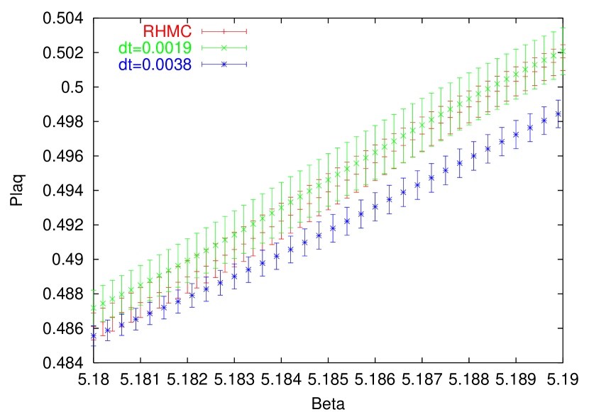
Figure 1: The plaquette behaviour near the chiral transition point (parameters given in Table 2).

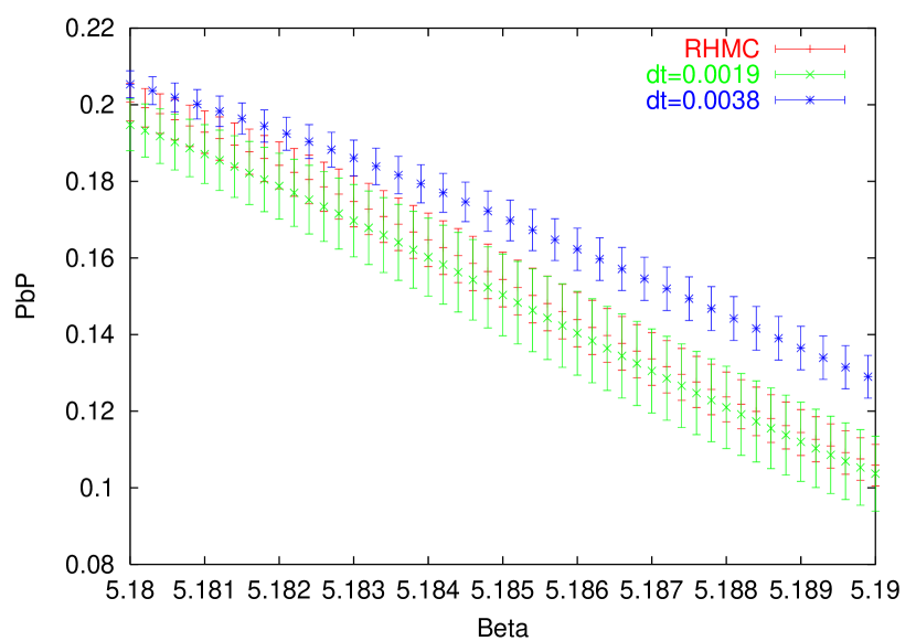
Figure 2: The $\bar{\psi}\psi$ behaviour near the chiral transition point (parameters given in Table 2).

Alg	$\delta\tau$	$A\%$	$B_{4}$
R	0.0019	-	1.56(5)
R	0.0038	-	1.73(4)
RHMC	0.055	$\approx 84$	1.57(2)

Table 1: Binder cumulant of $\langle\bar{\psi}\psi\rangle$, $B_{4}$, and RHMC acceptance rate $A$ from the finite temperature study ($2+1$ flavour naïve staggered fermions, Wilson gauge action, $V=8^{3}\times 4$, $m_{\mbox{\tiny ud}}=0.0076$, $m_{\mbox{\tiny s}}=0.25$, $\tau=1.0$)

Alg	$m_{\mbox{\tiny ud}}$	$m_{\mbox{\tiny s}}$	$\delta\tau$	$A$%	$P$
R	0.04	0.04	0.01	-	0.60812(2)
R	0.02	0.04	0.01	-	0.60829(1)
R	0.02	0.04	0.005	-	0.60817(3)
RHMC	0.04	0.04	0.02	65.5	0.60779(1)
RHMC	0.02	0.04	0.0185	69.3	0.60809(1)

Table 2: The different masses at which the domain wall results were gathered, together with the step-sizes $\delta\tau$, acceptance rates $A$ and plaquettes $P$ ($V=16^{3}\times 32\times 8$, DBW2 gauge action, $\beta=0.72$).

On each configuration the Binder cumulant was measured. The cumulant is important because it probes the strength of the phase transition. Only when R is using an integration step-size of $\delta\tau\leq m_{\mbox{\tiny ud}}/4$ is the step-size sufficiently small that the finite step-size errors are negligible (see Table 2). The correct value is obtained with RHMC using a step-size $\approx 29$ times larger: this represents a considerable improvement in efficiency.

4 2+1 Domain Wall Fermions

Again a comparison of R and RHMC was performed, but now using domain wall fermions with a more realistic volume (the parameters from this study are presented in Table 2). Applying RHMC to the case of domain wall fermions is not as trivial as for staggered fermions. The one flavour domain wall fermion determinant is given by $\left.\mathop{\rm det}\sqrt{M_{\mbox{\tiny PF}}^{\dagger}M_{\mbox{\tiny PF}}}\right/\mathop{\rm det}\sqrt{M_{\mbox{\tiny PV}}^{\dagger}M_{\mbox{\tiny PV}}}=\mathop{\rm det}\sqrt{{\cal M}^{\mbox{\tiny DWF}}}$. The additional Pauli-Villars bosonic determinant is required to cancel the heavy modes appearing in the bulk of the fifth dimension. Unfortunately, we cannot use $r({{\cal M}^{\mbox{\tiny DWF}}})$ as this would lead to a nested inversion in the solver. Therefore, the action is written $S_{\mbox{\tiny F}}=\bar{\phi}\left({M_{\mbox{\tiny PV}}^{\dagger}M_{\mbox{\tiny PV}}}\right)^{\mathchoice{\textstyle{1\over 2}}{\scriptstyle{1\over 2}}{\scriptscriptstyle{1/2}}{1/2}}\phi+\bar{\chi}\left({M_{\mbox{\tiny PF}}^{\dagger}M_{\mbox{\tiny PF}}}\right)^{-{\mathchoice{\textstyle{1\over 2}}{\scriptstyle{1\over 2}}{\scriptscriptstyle{1/2}}{1/2}}}\chi$, and now each matrix kernel can be written as a rational approximation. Thus we require 2 fermion fields to simulate a single flavour contribution. The naïve additional cost of this formulation is small ($m_{\mbox{\tiny PV}}\gg m_{\mbox{\tiny ud}}$), but is inherently more noisy because the heavy mode cancellation is only done stochastically. This results in larger forces, and a smaller step-size will be required than if the cancellation was exact [4] (the resolution to this problem shall be presented in §5.2). The R algorithm also uses stochastic cancellation, the bosonic Pauli-Villars field is included through the use of negative flavour number.

The step-size dependence of the plaquette is shown in Figure 4, from this extrapolation it is clear that to obtain a consistent result between the algorithms requires that R use an integration step-size at least 10 times smaller than RHMC.

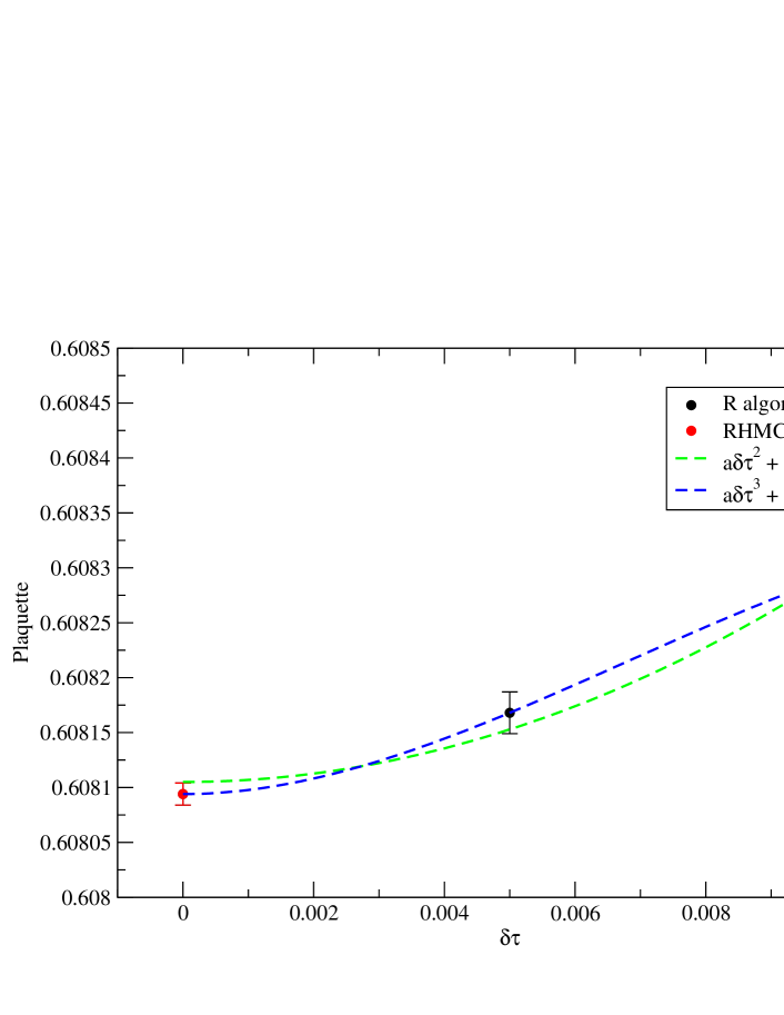
Figure 3: The step-size variation of the plaquette ($m_{\mbox{\tiny ud}}=0.02$, additional parameters given in Table 2).

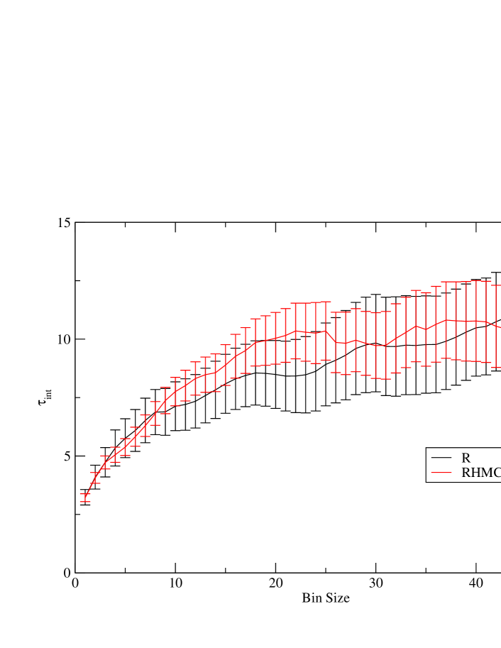
Figure 4: The integrated autocorrelation time of the $13^{\mbox{\rm\tiny th}}$ time-slice of the pion propagator ($m_{\mbox{\tiny ud}}=0.04$, parameters given in Table 2).

No algorithm comparison would be complete without a comparison of autocorrelations. In this study, both the plaquette and pion integrated autocorrelation times were measured, and it was found that there was very little to distinguish the two algorithms (see, e.g., Figure 4).

5 Improving RHMC

5.1 Integration Scheme

It has recently been shown [5], that the optimal second order symmetric symplectic integrator is not the leapfrog integrator, rather it is that given by Omelyan et al [6], which is given by

$$\hat{U}_{\mbox{\tiny QPQPQ}}(\delta\tau)=e^{\lambda\delta\tau Q}\;e^{\delta\tau P/2}\;e^{(1-2\lambda)\delta\tau Q}\;e^{\delta\tau P/2}\;e^{\lambda\delta\tau Q},$$

where $Q$ and $P$ represent the coordinate and momenta update operators respectively and $\lambda$ is a tuneable parameter whose optimal value is found to be $\lambda\approx 0.1931$. The Omelyan integrator is approximately double the cost of leapfrog, but theoretically should lead to a 3 fold improvement in conservation of the Hamiltonian: a net 50% gain. This integration scheme can of course be used with RHMC, and leads to a near 40% improvement in acceptance rate (see Table 5).

Integrator	$\delta\tau$	$A\%$
Leapfrog	0.02	63.6
Omelyan	0.04	88.8

Table 3: A comparison of the leapfrog and Omelyan integrators, using domain wall fermions ($V=16^{3}\times 32\times 8$, Iwasaki gauge action, $\beta=2.13$, $m_{\mbox{\tiny ud}}=m_{\mbox{\tiny s}}/2$).

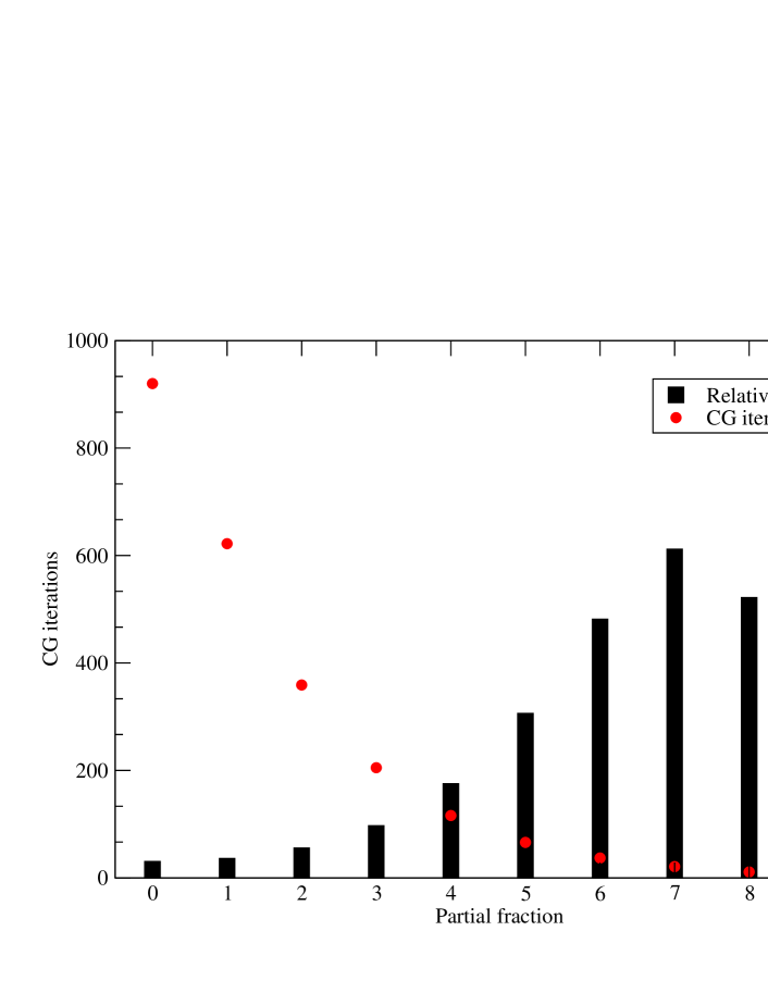
Figure 5: DWF Force magnitude ($\beta=2.13$, $m_{\mbox{\tiny ud}}/m_{\mbox{\tiny s}}=0.25$, $V=24^{3}\times 64\times 16$)

5.2 Exact Heavy Mode Cancellation

In the results presented in §4, the RHMC domain wall calculations were performed using only a stochastic cancellation of the heavy modes, and it was noted that this leads to larger fermion forces, hence a more costly algorithm. Since that study was conducted, a resolution to this problem has been found. The one flavour DWF determinant can be rewritten as

$$\sqrt{\frac{\mathop{\rm det}{M_{\mbox{\tiny PF}}^{\dagger}M_{\mbox{\tiny PF}}}}{\mathop{\rm det}{M_{\mbox{\tiny PV}}^{\dagger}M_{\mbox{\tiny PV}}}}}=\mathop{\rm det}\left[({M_{\mbox{\tiny PV}}^{\dagger}M_{\mbox{\tiny PV}}})^{-{\mathchoice{\textstyle{1\over 8}}{\scriptstyle{1\over 8}}{\scriptscriptstyle{1/8}}{1/8}}}({M_{\mbox{\tiny PF}}^{\dagger}M_{\mbox{\tiny PF}}})^{{\mathchoice{\textstyle{1\over 4}}{\scriptstyle{1\over 4}}{\scriptscriptstyle{1/4}}{1/4}}}({M_{\mbox{\tiny PV}}^{\dagger}M_{\mbox{\tiny PV}}})^{-{\mathchoice{\textstyle{1\over 8}}{\scriptstyle{1\over 8}}{\scriptscriptstyle{1/8}}{1/8}}}\right]^{2},$$

and the resulting pseudofermion action is given by

$$S_{\mbox{\tiny F}}=\bar{\phi}\left[({M_{\mbox{\tiny PV}}^{\dagger}M_{\mbox{\tiny PV}}})^{\mathchoice{\textstyle{1\over 4}}{\scriptstyle{1\over 4}}{\scriptscriptstyle{1/4}}{1/4}}({M_{\mbox{\tiny PF}}^{\dagger}M_{\mbox{\tiny PF}}})^{-{\mathchoice{\textstyle{1\over 2}}{\scriptstyle{1\over 2}}{\scriptscriptstyle{1/2}}{1/2}}}({M_{\mbox{\tiny PV}}^{\dagger}M_{\mbox{\tiny PV}}})^{\mathchoice{\textstyle{1\over 4}}{\scriptstyle{1\over 4}}{\scriptscriptstyle{1/4}}{1/4}}\right]^{2}\phi=\bar{\phi}\,\left[r_{1}({M_{\mbox{\tiny PV}}^{\dagger}M_{\mbox{\tiny PV}}})\,r_{2}({M_{\mbox{\tiny PF}}^{\dagger}M_{\mbox{\tiny PF}}})\,r_{1}({M_{\mbox{\tiny PV}}^{\dagger}M_{\mbox{\tiny PV}}})\right]^{2}\,\phi;$$

where $r_{1}(x)\approx x^{\mathchoice{\textstyle{1\over 4}}{\scriptstyle{1\over 4}}{\scriptscriptstyle{1/4}}{1/4}}$ and $r_{2}(x)\approx x^{-{\mathchoice{\textstyle{1\over 2}}{\scriptstyle{1\over 2}}{\scriptscriptstyle{1/2}}{1/2}}}$. The kernel that appears in the bilinear term is now in a form that allows heatbath evaluation (it is the square of a real positive operator) and a multi-shift solver can be used to evaluate each rational function that appears in the action. At each step of the MD trajectory three inversions are required compared to two for the stochastic formulation presented in §4. Since two of these inversions are using the Pauli-Villars matrix the cost of the extra inversion is negligible. This formulation should allow for large increases in the integration step-size. This shall be the subject of further study.

5.3 Fermion force tuning

The RHMC fermionic force given in equation (1) is just a sum of HMC-like force terms, each with different magnitude. Figure 5 is a plot showing the magnitude of the force associated with each shift. Also included is the number of conjugate gradient iterations required by the solver for each shift. The key point is that the most expensive shifts are also those which contribute least to the total fermion force. Since the acceptance rate is determined by the quantity $F\delta\tau$, this suggests that the small shifts can use a larger integration step-size than the large shifts. Hence, we could split the partial fractions into multiple timescales and use a multi-timescale integration scheme. An alternative strategy consists of relaxing the convergence of the multi-shift solver for the smaller shifts, but maintaining tight convergence for the larger shifts. An initial study into how much improvement can be gained from these strategies is currently being undertaken, it would appear that at least a factor of two can be gained, subject to further tuning.

6 Conclusions and outlook

In this work we have presented the exact RHMC algorithm and compared it to the inexact R algorithm in two regimes, namely near the chiral transition point of QCD using small volumes, and at low temperature using more realistic volumes. In both regimes, it was found that R must be run using a much smaller step-size than RHMC to achieve consistency between the two algorithms. Extrapolation of the R results to zero step-size is also significantly more expensive than just using RHMC. The conclusion therefore, is that there is no need for further use of the R algorithm.

Various improvements to the standard RHMC formulation were presented which lead to further performance improvements. It would be interesting to compare this improved RHMC to other exact algorithms, indeed this shall be the subject of future study.

7 Acknowledgements

We thank Chris Maynard and Rob Tweedie for help generating the datasets used in this work. We thank Peter Boyle, Dong Chen, Norman Christ, Saul Cohen, Calin Cristian, Zhihua Dong, Alan Gara, Andrew Jackson, Bálint Joó, Chulwoo Jung, Richard Kenway, Changhoan Kim, Ludmila Levkova, Xiaodong Liao, Guofeng Liu, Robert Mawhinney, Shigemi Ohta, Konstantin Petrov, Tilo Wettig, and Azusa Yamaguchi for developing with us the QCDOC machine and its software. This development and the resulting computer equipment used in this calculation were funded by the U.S. DOE grant DE-FG02-92ER40699, PPARC JIF grant PPA/J/S/1998/00756 and by RIKEN. This work was supported by PPARC grant PPA/G/O/2002/00465. Ph. de F. thanks the Minnesota Supercomputer Institute for computer resources.

References

- [1] S. A. Gottlieb, W. Liu, D. Toussaint, R. L. Renken and R. L. Sugar, Phys. Rev. D 35 (1987) 2531.
- [2] M. A. Clark, A. D. Kennedy and Z. Sroczynski, arXiv:hep-lat/0409133.
- [3] J. B. Kogut and D. K. Sinclair, arXiv:hep-lat/0504003.
- [4] Y. Aoki et al., arXiv:hep-lat/0411006.
- [5] T. Takaishi and P. de Forcrand, arXiv:hep-lat/0505020.
- [6] I. P. Omelyan, I. M. Mryglod and R. Folk, Comp. Phys. Comm. 151 (2003) 272.