A quenched study of $m_{b}$ in HQET beyond the leading order

Abstract:

A non perturbative method to compute the mass of the b quark including the $1/m$ term in HQET has been presented in [1]. Following this strategy, we find in the $\overline{\mbox{MS}}$ scheme $m_{\rm b}^{\rm stat}(m_{\rm b})=4.350(64)\,{\rm GeV}$ for the leading term, and $m_{\rm b}^{(1)}(m_{\rm b})=-0.049(29)\,{\rm GeV}$ for the next to leading order correction. This method involves several steps, including the simulation of the relativistic theory in a small volume, and of the effective theory in a big volume. Here we present some numerical details of our calculations.

PoS(LAT2005)224

1 Introduction

The b quark mass enters in the theoretical predictions of B mesons decay rates, which provide some of the most precise constraints in the unitarity triangle analysis. The Particle Data Group [2] quotes a value of $m_{\rm b}(m_{\rm b})$ between 4.1 and 4.4 GeV in the $\overline{\mbox{MS}}$ scheme, as the result of different determinations which include lattice computations.

On the lattice, heavy quarks are treated by using effective theories, in particular HQET when dealing with heavy-light systems. The b quark mass can then be predicted using the mass of the B meson as experimental input. In this framework, the bare parameters must be determined non perturbatively, in order to have a well defined continuum limit. This programme has been completed for the lowest order of the HQET (static theory) in the quenched approximation. The result from [3], $m_{\rm b}(m_{\rm b})=4.12(11)$ GeV is in reasonable agreement with [4], suggesting that the $1/m$ corrections to the b quark mass are small. Here we explicitly compute these corrections following the strategy proposed in [1]. This clearly represents an important test of HQET, which provides indications about its “convergence”.

The method relies on matching QCD and the effective theory in a small volume. The observables are then evolved to large volumes where contact with experiments can be established. Such an evolution is performed in the effective theory. Different systematics errors have to be controlled in the two regimes. For a precise matching in the small volume a very accurate determination of the relevant renormalization constants in the full theory is needed. On the other hand, in large volume simulations the main problems usually concern the separation of the ground state from the excited states.We present details on the numerical evaluation of the various ingredients entering the computation of the $1/m$ corrections to the b quark mass. The increase in the (numerical) effort is moderate compared to the static case. A related investigation is described in [5].

2 Finite volume

2.1 Relativistic part

The observables $\Phi_{1,2}$ are defined as in eqs.  (I.2.5), (I.2.6) by ($T=L/2$)

$$\Phi_{1}(L,M)= \Phi_{1}^{\rm rel}(L,M)+\Phi_{1}^{\rm stat}(L)\quad\mbox{and}\quad\Phi_{2}(L,M)={L\over{2a}}\ln\left({f_{1}^{\rm av}(T-a)\over f_{1}^{\rm av}(T+a)}\right)\quad$$ (1)

where $$\Phi_{1}^{\rm rel}(L,M)= \ln\left({f_{1}^{\rm av}(\theta,T)\over f_{1}^{\rm av}(\theta^{\prime},T)}\right)\qquad\mbox{and}\qquad\Phi_{1}^{\rm stat}(L)=-\ln\left({f_{1}^{\rm stat}(\theta,T)\over f_{1}^{\rm stat}(\theta^{\prime},T)}\right)\,.$$ (2)

The observables $\Phi_{1}^{\rm rel}$ and $\Phi_{2}$ are computed in (quenched) QCD, with the O($a$)-improved Wilson action as in [6]. The light quark mass is fixed to be zero. While we use different resolutions $L_{1}/a=20,24,32,40$, the physical size of the lattice is kept fixed by determining the bare coupling such that the SF coupling is  $\bar{g}^{2}(L_{1}/4)=1.88$ [7, 6]. Using $r_{0}=0.5\,{\rm fm}$ to convert to physical units, one finds $L_{1}\approx 0.36$ fm. We take three different values $\theta,\theta^{\prime}=0,\ 0.5,\ 1$ for the periodicity phases. We want to interpolate our data to the b quark mass, and since according to [3], the value of $L_{1}M_{\rm b}^{\rm RGI}$ is around 12, we simulate three different values of $z=L_{1}M$ : $10.3,12,13.2$. For each of these values $\Phi_{2}(L_{1},M)$ is extrapolated to the continuum via a linear fit in $(a/L_{1})^{2}$ using only the lattices of resolution $L_{1}/a=24,32,40$. We confirmed that adding the coarsest lattice does not change the values of the continuum limit, as one can also see in fig. 1. We then fit the continuum values - see also eq. (I.5.5) - to the following form

$$\Phi_{2}(L_{1},M)=\mbox{Const}+S\times L_{1}M\,,$$ (3)

to find the slope $S=0.61(5)$. At this point, we note that a source of error originates from the determination [6] of the (universal) renormalization factor $M_{\rm b}^{\rm RGI}/{\overline{m}_{\rm SF}(1/L_{0})}$. It amounts to a one percent uncertainty on $\Phi_{2}$.

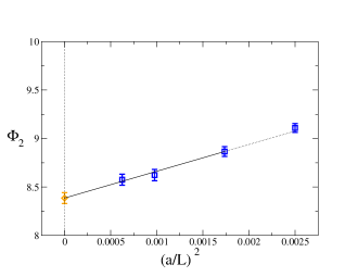
Figure 1: Continuum extrapolation of $\Phi_{2}$, for $L_{1}M=12$

2.2 Effective theory

Using the static actions denoted by HYP1 and HYP2 in [8], we compute boundary to boundary correlation functions of the QCD Schrödinger functional, but now in the effective theory and for two values of $L$. The smaller one is again $L=L_{1}$, but with the resolutions $L_{1}/a=6,8,10,12$, corresponding to $\beta=\ 6.2204,\ 6.476,\ 6.635,\ 6.775\$ respectively and the larger one is $L=L_{2}=2L_{1}$ with the same values of $a$. As we did for the relativistic part, for each of these volumes and resolutions, the simulations are done with three values of the time extent, namely $T=\ L/2,\ L/2-a,\ L/2+a$, and three values of the periodicity angles. Following [1], we compute $f_{1}^{\rm stat}$ and $f_{1}^{\rm kin}$ for these different sets of parameters and from those the functions $\Gamma_{1}^{\rm stat}$, $\Gamma_{1}^{\rm kin}$ and $R_{1}^{\rm kin}$ as they are defined in eqs. (I.2.8 - I.2.10) – at finite values of the lattice spacing.

3 Step scaling functions

Once we have the quantities described in the previous section, we compute the step scaling functions $\sigma_{m}$, $\sigma_{1,2}^{\rm kin}$, defined as in eqs (I.3.1 - I.3.3). At finite lattice spacing, we have

$$\Sigma_{m}(u,a/L_{1}) = 2L_{1}\left[\Gamma_{1}^{\rm stat}(2L_{1},a)-\Gamma_{1}^{\rm stat}(L_{1},a)\right]_{u=\bar{g}^{2}(L_{1})}$$ (4)

$$\Sigma_{1}^{\rm kin}(u,a/L_{1})=\left.{R^{\rm kin}_{1}(2L_{1},a)\over R^{\rm kin}_{1}(L_{1},a)}\right|_{u=\bar{g}^{2}(L_{1})}\quad\Sigma_{2}^{\rm kin}(u,a/L_{1})=2L_{1}\left.{{\Gamma^{\rm kin}_{1}(2L_{1},a)-\Gamma^{\rm kin}_{1}(L_{1},a)}\over{R^{\rm kin}_{1}(L_{1},a)}}\right|_{u=\bar{g}^{2}(L_{1})}.\hskip 14.22636pt$$ (5)

Their continuum limits

$$\sigma_{m}(u)=\lim_{a/L_{1}\rightarrow 0}\Sigma_{m}(u,a/L_{1})\qquad\sigma_{1,2}^{\rm kin}(u)=\lim_{a/L_{1}\rightarrow 0}\Sigma_{1,2}^{\rm kin}(u,a/L_{1})$$ (6)

are well defined. Since the static theory is O($a$)-improved, $\sigma_{m}(u)$ is obtained by a linear fit in $(a/L_{1})^{2}$, and we choose to use only the two finest lattices, corresponding to $L_{1}/a=10,12$ . The kinetic step scaling functions $\sigma_{1,2}^{\rm kin}(u)$ are extracted by fitting the data of the three finer lattices linearly in $a/L$. Both for $\Sigma_{1}^{\rm kin}$ and for $\Sigma_{\rm m}$ we could have included one coarser lattice without a significant change (apart from smaller errors) as illustrated in figs. 2,3. 

Since we find well compatible results from the different actions after taking the continuum limits, we choose a constrained fit in the final analysis. In that case, the error is computed by a jackknife procedure, binning the data in such a way that the number of jackknife configurations is the same for the different sets of data. We note that a very significant $\theta,\theta^{\prime}$ dependence is still left in the kinetic step scaling functions (I.2.8), nevertheless the final physical results will turn out to be independent of these kinematical variables as they should (apart from small $1/m^{2}$ terms). In our figures, we made the choice $(\theta,\theta^{\prime})=(0,0.5)$.

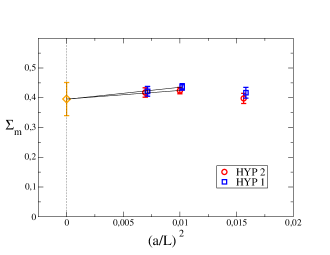
Figure 2: Continuum extrapolation of the static step scaling function

4 Large volume

The quantities computed in “infinite” volume are the static and the kinetic energy (I.4.2), where now the light quark mass is fixed to $m_{\mathrm{strange}}$. These energies occur in eq. (I.4.1), through the terms $[E^{\rm stat}-\Gamma_{1}^{\rm stat}(L_{2})]$ and $[\omega_{\rm kin}({\hat{E}}^{\rm kin}-\Gamma_{1}^{\rm kin}(L_{2}))]$ . The infinite and the finite volume part of the static and the kinetic energy are of course computed at the same value of the lattice spacing (in order to cancel the divergences, as we did for the step scaling function). Our approximation to infinite volume is $L_{\infty}=4L_{1}\simeq 1.5$ fm (again using $r_{0}=0.5\,{\rm fm}$), and we use two resolutions $L_{\infty}/a=16,24$, corresponding to $\beta=6.0219\,,\;6.2885$ respectively. We obtain a nice signal for $E_{\rm stat}$ due to the HYP1/2 actions [8]. The errors in the effective mass remain below a level of few MeV out to 2 fm time separation. Thus the significant excited state contamination can be removed with confidence and $E^{\rm stat}-\Gamma_{1}^{\rm stat}(L_{2})=612(2)\,{\rm MeV}$ and $597(2)\,{\rm MeV}$ are found at $\beta=6.0219\,,\;6.2885$ respectively for the action HYP2. From this we quote at present $E^{\rm stat}-\Gamma_{1}^{\rm stat}(L_{2})=586(11){\rm MeV}$ as a continuum number.

However, $[\omega_{\rm kin}({\hat{E}}^{\rm kin}-\Gamma_{1}^{\rm kin}(L_{2}))]$ is very small and the errors of the effective ($x_{0}$-dependent) ${\hat{E}}^{\rm kin}$ grow rather rapidly with $x_{0}$. Thus, although we will see that this error is not dominant in the end, $[\omega_{\rm kin}({\hat{E}}^{\rm kin}-\Gamma_{1}^{\rm kin}(L_{2}))]$ has a large relative error.

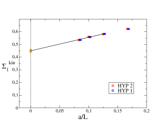
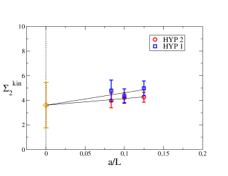
Figure 3: Continuum extrapolation of the kinetic step scaling functions

5 The RGI b quark mass

5.1 Static part

The value of the RGI quark mass in the static approximation, defined by eq. (I.5.4), is obtained by a linear interpolation of (I.5.2), where we used $m_{\rm B}^{experimental}=5404$ MeV as appropriate for a strange quark. This interpolation is illustrated in fig 4. We obtain (the conversion to physical units is done with $r_{0}=0.5\,{\rm fm}$)

$$r_{0}M_{\rm b}^{\rm stat}=\left\{\begin{array}[]{ll}17.18(25)\mbox{ (HYP2)}\\ 17.15(25)\mbox{ (HYP1)}\end{array}\right.\qquad M_{\rm b}^{\rm stat}=\left\{\begin{array}[]{ll}6771(99)\mbox{ MeV (HYP2)}\\ 6757(99)\mbox{ MeV (HYP1)}\end{array}\right.$$ (11)

5.2 $1/m$ corrections

The next to leading order correction of the b quark mass can be separated in two parts, corresponding to $m_{\rm B}^{\rm(1a)}$, computed entirely from the small volume, and $m_{\rm B}^{\rm(1b)}$, given by eq. (I.5.3). Following eq. (I.5.6) we have

$$M_{\rm b}^{\rm(1a)} = -{1\over S}\sigma^{\mathrm{kin}}_{2}(\bar{g}^{2}(L_{1}))\Phi_{1}(L_{1},M_{\rm b}^{\rm stat})$$ (12)

$$M_{\rm b}^{\rm(1b)} = -{1\over S}\left[L_{2}\,(\hat{E}^{\mathrm{kin}}-\Gamma^{\rm kin}_{1}(L_{2}))\omega_{\mathrm{kin}}\right],$$ (13)

and we find for the action HYP2

$$\begin{array}[]{||c|c||c|c||}\hline\cr\hline\cr\theta&\theta^{\prime}&r_{0}M_{\rm b}^{\rm(1a)}&r_{0}M_{\rm b}^{\rm(1b)}\\ \hline\cr\ \ 0&\ \ 0.5&\quad-0.08(4)&\quad-0.14(11)\\ \ \ 0.5&\ \ 1&\quad-0.08(4)&\quad-0.15(11)\\ \ \ 1&\ \ 0&\quad-0.08(4)&\quad-0.15(11)\\ \hline\cr\hline\cr\end{array}$$ (18)

while for HYP1 the numbers are compatible but have larger uncertainties. It is now clear that the results are $\theta,\theta^{\prime}$-independent. In physical units, we find the scale and scheme independent numbers

$$M_{\rm b}^{\rm(1a)}=-30(15)\ {\rm MeV}\qquad M_{\rm b}^{\rm(1b)}=-56(43)\ {\rm MeV}$$ (19)

in the quenched approximation.

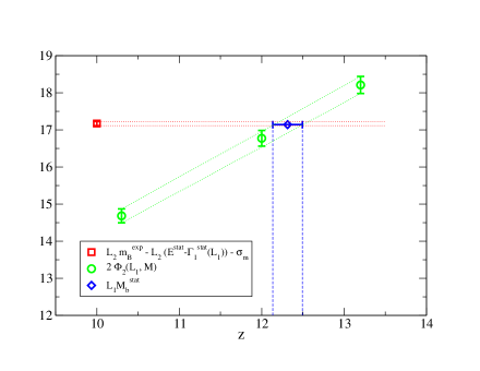
Figure 4: Interpolation and solution of eq. (I.5.2)

6 Conclusions

Our numerical results show that indeed the $1/m$ corrections can be computed with a precision which is – at present – better than the one of the leading (static) result: the absolute errors of leading and next-to-leading terms are in a ratio of about two to one. This is a first demonstration of the practicability of the strategy of [3] beyond the leading order. Still, as mentioned in the previous section, the errors of correlation functions with the kinetic insertion grow rather rapidly in time and when decreasing the lattice spacing. The former behavior is at present not understood.

The size of the $1/m$ corrections $M_{\rm b}^{\rm(1a)}$ and $M_{\rm b}^{\rm(1b)}$ is small and confirms the validity of the naive counting in terms of powers of $\Lambda/m_{{\rm b}}$. Further numerical confirmation of this is provided by the close agreement of our result with the one - also in quenched QCD - of [4], $r_{0}M_{\rm b}=17.08(41)$ where the effective theory was not used. This also means that $1/m^{2}$ terms can be neglected altogether.

On the other hand, our static result differs (statistically) significantly from the static one of [3], $r_{0}M_{\rm b}=16.12(25)(15)$, where the second error is in common between that computation and the present one. In [3] the matching was performed using an other observable, and at $L=L_{0}=L_{1}/2$. By a comparison to our present NLO result, we see that this leads to a somewhat larger ($\simeq 5\%$) $1/m$ correction. This is not at all unexpected, cf. item 3 in section 6 of [1]. In fact, an explicit computation of this correction would be another interesting confirmation of the applicability of the effective theory.

Let us finally translate our numbers to the ${\rm\overline{MS\kern-0.50003pt}\kern 0.50003pt}$ scheme. With $r_{0}=0.5\,{\rm fm}$ and $\Lambda_{\rm\overline{MS\kern-0.35002pt}\kern 0.35002pt}^{(0)}=238\,{\rm MeV}$ [7] we find for the b quark mass at its own scale

$$m_{\rm b}=m_{\rm b}^{\rm stat}+m_{\rm b}^{(1)}\,,\qquad m_{\rm b}^{\rm stat}(m_{\rm b})=4.350(64)\,{\rm GeV}\,,\quad m_{\rm b}^{(1)}(m_{\rm b})=-0.049(29)\,{\rm GeV}\,.$$ (20)

Despite the employed quenched approximation, the total result, $m_{\rm b}(m_{\rm b})=4.30(7)\,{\rm GeV}$, is in good agreement with the range quoted in the particle data book and not far from the precise value of $m_{\rm b}(m_{\rm b})=4.19(5)\,{\rm GeV}$ derived in [9] from the $e^{+}e^{-}\to b$ total cross section and high order perturbation theory. Our result is also compatible with the early computation (quenched and static) of [10] $m_{\rm b}(m_{\rm b})=4.41(5)(10)\,{\rm GeV}$, where the matching was done perturbatively at the NLO. This last result was updated to 4.30(5)(5) GeV in [11] with the help of the NNLO result of [12].

It seems that on the one hand it is the right time to apply these methods both to quantities where larger $1/m$ corrections are expected, such as $F_{\rm B}$, and to the mass of the b quark in full QCD. On the other hand, research should continue to improve the statistical errors in particular of the $1/m$ corrections in large volume. A promising route is to follow [13, 14].

Acknowledgement. We thank NIC for allocating computer time on the APEmille computers at DESY Zeuthen to this project and the APE group for its help.

References

- [1] ALPHA, M. Della Morte, N. Garron, M. Papinutto and R. Sommer, PoS (2005) 223, hep-lat/0509084.
- [2] Particle Data Group, E. S. et al., Phys. Lett. B592 (2004) 1.
- [3] ALPHA, J. Heitger and R. Sommer, JHEP 02 (2004) 022, hep-lat/0310035.
- [4] G.M. de Divitiis, M. Guagnelli, R. Petronzio, N. Tantalo and F. Palombi, Nucl. Phys. B675 (2003) 309, hep-lat/0305018.
- [5] S. Negishi, H. Matsufuru, T. Onogi and T. Umeda, PoS (2005) 208, hep-lat/0510048.
- [6] ALPHA, J. Heitger and J. Wennekers, JHEP 02 (2004) 064, hep-lat/0312016.
- [7] ALPHA, S. Capitani, M. Lüscher, R. Sommer and H. Wittig, Nucl. Phys. B544 (1999) 669, hep-lat/9810063.
- [8] M. Della Morte, A. Shindler and R. Sommer, JHEP 08 (2005) 051, hep-lat/0506008.
- [9] J.H. Kühn and M. Steinhauser, Nucl. Phys. B619 (2001) 588, hep-ph/0109084.
- [10] G. Martinelli and C.T. Sachrajda, Nucl. Phys. B559 (1999) 429, hep-lat/9812001.
- [11] V. Lubicz, Nucl. Phys. Proc. Suppl. 94 (2001) 116, hep-lat/0012003.
- [12] F. Di Renzo and L. Scorzato, JHEP 02 (2001) 020, hep-lat/0012011.
- [13] J. Foley et al., hep-lat/0505023.
- [14] SESAM, G.S. Bali, H. Neff, T. Duessel, T. Lippert and K. Schilling, Phys. Rev. D71 (2005) 114513, hep-lat/0505012.