Real-time dynamics of proton decay

Abstract:

Substituting Skyrmion for nucleon, one can potentially see — in real time — how the monopole is catalysing the proton (or neutron) decay, and even obtain a plausible estimate for catalysis cross-section. Here we discuss the key aspects of a practical implementation of such approach and demonstrate how one can overcome the main technical problems: Gauss constraint violation and reflections at the boundaries.

PoS(LAT2005)313

1 Introduction

The monopole catalysis of proton decay [1, 2] is a complicated process involving several different physical scales. Although the physics of how fermions interact with the monopole is rather well understood, the net proton decay cross-section remains unknown, mainly because the proton decay actually happens via a combination of quite different physical mechanisms. At first, spatially separated monopole and proton interact at relatively large distances; then, the monopole starts to interact with individual quark states inside the proton, whose internal structure is defined by non-perturbative QCD phenomena.

An interesting possibility to study both kinds of processes is provided [3] by the Skyrme theory [4]. However, even though the monopole catalysis of the Skyrmion decay is essentially a classical process, its cross-section is also not known. Recently it has been suggested [5, 6] to study this process in a system of the Skyrmion interacting with the ’t Hooft-Polyakov monopole [7, 8]. Since the latter is a spatially extended object, this makes the model free from singularities and greatly simplifies its numerical study. In the papers [5, 6], the spherically-symmetric monopole-Skyrmion geometry has been comprehensively studied in quasistatic limit. In particular, the decay path of the Skyrmion has been identified, and it has been shown that nothing prevents the Skyrmion from promptly losing almost all of its energy in the monopole background.

The natural next step is to study the classical dynamics of the model suggested in [5, 6]. In this talk we discuss the main technical aspects of such a study, while the physical results will be published elsewhere [10]. In particular, we concentrate on a problem of gauge invariance violation in real-time classical simulations.

2 The model

The model consists of the Skyrme field $U$ coupled to two gauge fields $A_{\mu}$ (group $SU(2)_{L}$) and $B_{\mu}$ (group $SU(2)_{R}$). The Higgs sector has two Georgi-Glashow Higgs fields $\Phi_{A}$ and $\Phi_{B}$ which break the $SU(2)_{L}$ and $SU(2)_{R}$ symmetries down to $U(1)_{L}$ and $U(1)_{R}$, respectively, and a third Higgs field $\Psi$ which breaks the axial subgroup of the remaining $U(1)_{L}\times U(1)_{R}$. These requirements fix the scalar field group representations completely: $U\in SU(2)$ , $U,\Psi:\;\;({\bf 2},{\bf\bar{2}})$, $\Phi_{A}:\;\;({\bf 3},{\bf 1})$, $\Phi_{B}:\;\;({\bf 1},{\bf 3})$.

The action for the model is

$$S = \int~{}d^{4}x~{}\left[-\frac{1}{2g^{2}}\mbox{Tr}(F_{\mu\nu}^{2})-\frac{1}{2g^{2}}\mbox{Tr}(G_{\mu\nu}^{2})\right]$$ (1)

$$- \int~{}d^{4}x~{}\left[\frac{1}{2}\mbox{Tr}(D_{\mu}\Phi_{A})^{2}+\frac{1}{2}\mbox{Tr}(D_{\mu}\Phi_{B})^{2}\right]$$

$$- \int~{}d^{4}x~{}\left[\frac{\lambda}{4}\left(\frac{1}{2}\mbox{Tr}(\Phi_{A}^{2})+v^{2}\right)^{2}+\frac{{\lambda}}{4}\left(\frac{1}{2}\mbox{Tr}(\Phi_{B}^{2})+v^{2}\right)^{2}\right]$$

$$+ \int~{}d^{4}x~{}\left[\frac{1}{2}\mbox{Tr}(D_{\mu}\Psi^{\dagger}D_{\mu}\Psi)+\frac{\tau}{4}\left(\frac{1}{2}\mbox{Tr}(\Psi^{\dagger}\Psi)-\zeta^{2}\right)^{2}\right]$$

$$+ \int~{}d^{4}x~{}\left[-\frac{F_{\pi}^{2}}{16}\mbox{Tr}(U^{\dagger}D_{\mu}U)^{2}+\frac{1}{32e^{2}}\mbox{Tr}([U^{\dagger}D_{\mu}U,U^{\dagger}D_{\nu}U]^{2})\right]$$

$$+ \Gamma_{WZW}$$

Here $F_{\mu\nu}$ and $G_{\mu\nu}$ are the field strengths of $A_{\mu}$ and $B_{\mu}$, the fields $\Phi_{A}$ and $\Phi_{B}$ are $2\times 2$ matrices from the algebras of $SU(2)_{L}$ and $SU(2)_{R}$, respectively,

$$D_{\mu}U = \partial_{\mu}U+A_{\mu}U-UB_{\mu}$$

$$D_{\mu}\Phi_{A} = \partial_{\mu}\Phi_{A}+[A_{\mu},\Phi_{A}]$$

$$D_{\mu}\Phi_{B} = \partial_{\mu}\Phi_{B}+[B_{\mu},\Phi_{B}]$$ (2)

and $F_{\pi}$ and $e$ are the pion decay constant and the Skyrme constant. The new Higgs field $\Psi$ is a $2\times 2$ complex matrix with covariant derivative identical to that of the Skyrme field,

$$D_{\mu}\Psi=\partial_{\mu}\Psi+A_{\mu}\Psi-\Psi B_{\mu}$$

Finally, the Wess–Zumino–Witten term $\Gamma_{WZW}$ can be safely ignored [5] in what follows.

The most general spherically symmetric Ansatz consistent with the symmetries [5, 6] of the action (1) is

$$A_{0} = -B_{0}=-{i\over 2}\left(\frac{a_{0}(r)}{r}\right)\hat{x}\cdot\vec{\sigma}$$

$$A_{i} = -{i\over 2}\left[\left(\frac{a_{1}(r)-1}{r}\right)\varepsilon_{ijk}\sigma_{j}\hat{x}_{k}+\left(\frac{a_{2}(r)}{r}\right)(\sigma_{i}-\hat{x}_{i}\hat{x}\cdot\vec{\sigma})+\left(\frac{a_{3}(r)}{r}\right)\hat{x}_{i}\hat{x}\cdot\vec{\sigma}\right]$$

$$B_{i} = -{i\over 2}\left[\left(\frac{a_{1}(r)-1}{r}\right)\varepsilon_{ijk}\sigma_{j}\hat{x}_{k}-\left(\frac{a_{2}(r)}{r}\right)(\sigma_{i}-\hat{x}_{i}\hat{x}\cdot\vec{\sigma})-\left(\frac{a_{3}(r)}{r}\right)\hat{x}_{i}\hat{x}\cdot\vec{\sigma}\right]\>$$

$$\Phi_{A} = \Phi_{B}=ivh(r)\hat{x}\cdot\vec{\sigma}$$

$$U = 1{\rm I}\cos f(r)+i\hat{x}\cdot\vec{\sigma}\sin f(r)\;\;\;,\;\;\;\Psi=\zeta[ih_{1}(r)\hat{x}.\sigma+h_{2}(r)1{\rm I}]$$ (3)

where $\hat{x}$ is the unit radius-vector.

Substituting the ansatz (3) into (1) and using the $A_{0}=B_{0}=0$ gauge to get the proper Hamilton real-time evolution, one obtains spherically-symmetric action which remains invariant to the following static gauge transformations which are the remains of the axial $U(1)$:

$$h_{2}+ih_{1} \to (h_{2}+ih_{1})e^{i\alpha(r)}$$

$$a_{1}+ia_{2} \to (a_{1}+ia_{2})e^{i\alpha(r)}$$

$$a_{3} \to a_{3}+r\partial_{r}\alpha(r)$$

$$f \to f+\alpha(r)$$ (4)

(note that $h_{2}+ih_{1}$ rotates identically to $e^{if}$, once the fields $\Psi$ and $U$ are in the same group representation). This remaining gauge invariance becomes a major obstacle in real-time simulations (see below).

The classical equations of motion can be obtained from the spherically-symmetric action by the standard variational procedure. Of particular importance for what follows is the Gauss constraint corresponding to variation over $a_{0}$:

$$\Delta=-\frac{1}{2g^{2}}\left[\partial_{r}\dot{a}_{3}+\frac{\dot{a}_{3}}{r}\right]+\frac{a_{1}\dot{a}_{2}-a_{2}\dot{a}_{1}}{g^{2}r}+\left[\frac{F_{\pi}^{2}}{8}r^{2}+\frac{1}{8e^{2}}(a_{1}\sin f-a_{2}\cos f)^{2}\right]\frac{\dot{f}}{r}-\zeta^{2}r(h_{1}\dot{h}_{2}-h_{2}\dot{h}_{1})=0$$ (5)

The constraint (5) is preserved by the equations of motion as long as their gauge invariance is not violated.

3 Numerical study

In the $A_{0}=B_{0}=0$ gauge the classical equations of motion obtainable from the action (1) represent a system of 2^nd-order hyperbolic partial differential equations in (1+1) dimensions which can be solved numerically by e.g. a staggered leapfrog scheme. Choosing different initial configurations, one can study several physically interesting cases of the Skyrmion decay. For example, starting from a normal vacuum Skyrme solution (so-called “bare” Skyrmion, see [5, 6]), one can simulate the decay of a physical nucleon. By choosing the initial profile for $f(r)$ corresponding to the “thin” Skyrmion (a static solution [5, 6] with unit baryon charge and minimal energy in the monopole background), it becomes possible to check [10] how close is its actual decay path to the quasistatic paths found in the Refs.[5, 6]. However, any such study is facing two serious difficulties related to the lack of gauge-invariant lattice action for the model and the need for fully absorbing boundary conditions.

3.1 Lattice action

To preserve the physical structure of continuum theory, its symmetries must be retained in the discretised lattice version, and, in particular, the symmetries to local gauge transformations. Unfortunately, we are not aware of any gauge-invariant lattice action for gauged Skyrme models, including the model used in the present study. The use of gauge-noninvariant lattice action, generally speaking, results in domination of nonphysical states in generated field configurations. However, in real-time classical evolution the mixing of physical and nonphysical states can be rather well controlled.

Since the only reason for gauge invariance violation are the discretisation errors, for reasonably small lattice spacing the magnitude of the violation remains rather small. Assuming that the evolution starts from a physical state which obeys the Gauss constraint (5), the system initially stays close to the physical manifold and can be projected back onto it after certain amount of time. Physically, the projection procedure involves the minimisation of the quantity

$$Q=\int dx\;\Delta^{2}$$ (6)

where $\Delta$ is the constraint value (the left-hand side of (5)). Generally speaking, any minimisation technique can be used here, with no specific approach favoured by physical reasons as long as the accumulated constraint violation remains small. In the present study we use a variation [9] of the steepest descent method, also called sometimes as the Langevin cooling.

It is worth noting that in real-time classical simulations the projection procedure is inevitable [9] even with a perfectly gauge-invariant lattice action. The reason is that the gauge invariance will inevitably be broken by computer roundoff errors. Even though the latter remain tiny ($O(10^{-15})$ for the standard double precision), the constraint violation accumulates in the course of evolution, which results in exponential divergency of constraints. To remain close to the physical manifold for indefinite period of time, one still has to periodically project the system onto it, although for gauge-invariant lattice schemes the constraint violation can be maintained at dramatically lower level.

Failure to keep constraint violation under control inevitably leads to an explosion of the numerical scheme, whether a gauge-invariant one or not. For the model at hand this is demonstrated at the Figure 1, where the system energy is plotted against the time along with the magnitude of the volume-averaged constraint value $<\Delta>_{\rm vol}$.

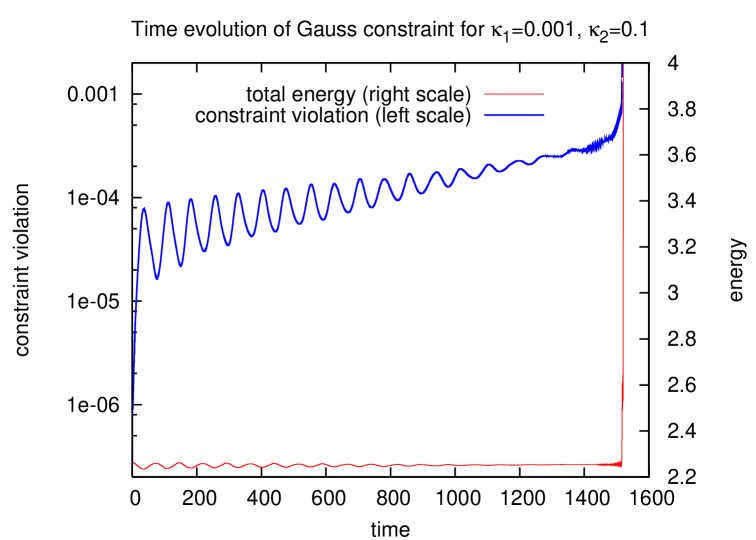
Figure 1: Constraint violation inevitably breaks stability of the numerical evolution, with the Gauss constraint and total energy exploding simultaneously after the former exceeds a certain critical level. Of course, the numerical scheme also violates the energy conservation (as demonstrated by the small oscillations of energy), but in non-gauge models [11] this doesn’t break the stability. Notations: $\kappa_{1}=F_{\pi}^{2}/8v^{2}$, $\kappa_{2}=g^{2}/64e^{2}$; for dimensionless units used see Ref.[6].

3.2 Absorption at the boundaries

In physical case, the energy of the decaying proton is released to the spatial infinity. In numerical studies, this energy should be either absorbed at the boundaries or allowed to pass through the boundaries. For massless waves this can be easily implemented by the standard outgoing-wave boundary conditions. However, in more realistic cases, including the present study, it turns out to be very difficult to achieve full absorption at the boundaries, simply because any modification of the theory near the boundaries introduces spatial inhomogeneities which scatter the waves back to centre. Fortunately, in (1+1)-dimensional case it is still possible to overcome the problem by brute force, taking a sufficiently large physical volume, so that the reflected wave wouldn’t come back to the origin before the end of the run, but this obviously cannot be done for higher spatial dimensions.

4 Conclusions

Despite the problems discussed above, the monopole catalysis of Skyrmion decay can be successively studied [10] in the spherically-symmetric case where one can determine the decay time of the Skyrmion when it is exactly overlapped with the monopole. In two spatial dimensions, one can study Skyrmion-monopole collisions at zero impact parameter; however, the catalysis cross-section can be established only by studying full-3D geometry. This is a major challenge, taking into account that the Skyrme dynamics is known [12]–[14] to become unstable already in 2D simulations, and a number of similar problems such as full numerical study of Skyrmion-anti-Skyrmion annihilation remain so far unsolved.

5 Acknowledgements

This work is done in collaboration with Y. Brihaye, V A. Rubakov and D. H. Tchrakian.

References

- [1] V. A. Rubakov, Superheavy Magnetic Monopoles And Proton Decay, JETP Lett. 33 (1981) 644 [Pisma Zh. Eksp. Teor. Fiz. 33 (1981) 658]; Adler-Bell-Jackiw Anomaly And Fermion Number Breaking In The Presence Of A Magnetic Monopole, Nucl. Phys. B 203 (1982) 311.
- [2] C. G. Callan, Disappearing Dyons, Phys. Rev. D 25 (1982) 2141; Dyon - Fermion Dynamics, Phys. Rev. D 26 (1982) 2058; Monopole Catalysis Of Baryon Decay, Nucl. Phys. B 212 (1983) 391.
- [3] C. G. Callan and E. Witten, Monopole Catalysis Of Skyrmion Decay, Nucl. Phys. B 239 (1984) 161.
- [4] T. H. Skyrme, A Nonlinear Field Theory, Proc. Roy. Soc. Lond. A 260 (1961) 127.
- [5] Y. Brihaye, V. A. Rubakov, D. H. Tchrakian and F. Zimmerschied, A simplified model for monopole catalysis of nucleon decay, Theor. Math. Phys. 128 (2001) 1140 [Teor. Mat. Fiz. 128 (2001) 361] [hep-ph/0103228].
- [6] Y. Brihaye, D. Yu. Grigoriev, V. A. Rubakov and D. H. Tchrakian, An extended model for monopole catalysis of nucleon decay, Phys. Rev. D 67 (2003) 034004 [hep-th/0211215].
- [7] G. ’t Hooft, Magnetic Monopoles In Unified Gauge Theories, Nucl. Phys. B 79 (1974) 276.
- [8] A. M. Polyakov, Particle Spectrum In Quantum Field Theory, JETP Lett. 20 (1974) 194 [Pisma Zh. Eksp. Teor. Fiz. 20 (1974) 430].
- [9] D. Yu. Grigoriev, V. A. Rubakov and M. E. Shaposhnikov, Topological Transitions At Finite Temperatures: A Real Time Numerical Approach, Nucl. Phys. B 326 (1989) 737.
- [10] Y. Brihaye, D. Yu. Grigoriev, V. A. Rubakov and D. H. Tchrakian, to be published.
- [11] D. Yu. Grigoriev and V. A. Rubakov, Soliton Pair Creation At Finite Temperatures. Numerical Study In (1+1)-Dimensions, Nucl. Phys. B 299 (1988) 67.
- [12] A. E. Allder, S. E. Koonin, R. Seki and H. M. Sommermann, Dynamics Of Skyrmion Collisions In (3+1)-Dimensions, Phys. Rev. Lett. 59 (1987) 2836.
- [13] W. Y. Crutchfield and J. B. Bell, Instabilities of the Skyrme model, J. Comput. Phys. 110 (1994) 234.
- [14] R. A. Battye and P. M. Sutcliffe, Multi-soliton dynamics in the Skyrme model, Phys. Lett. B 391 (1997) 150 [hep-th/9610113].