Four-loop plaquette in 3d with a mass regulator

Abstract:

The QCD free energy can be studied by dimensional reduction to a three-dimensional (3d) effective theory, whereby non-perturbative lattice simulations become less demanding. To connect to the original QCD a perturbative matching computation is required, which is conventionally carried out in dimensional regularization. Therefore the 3d lattice results need to be converted to this regularization scheme as well. The conversion must be carried up to 4-loop order, where the free energy displays an infrared (IR) singularity. We therefore need a regulator which can be implemented both on the lattice and in the continuum computation. We introduce a mass regulator to perform Numerical Stochastic Perturbation Theory computations. Covariant gauge is fixed in the Faddeev-Popov scheme without introducing any ghost fields.

PoS(LAT2005)189

1 Introduction

As is well known, finite-temperature QCD seems to show two different phases: it is confining at low temperatures (the realm of mesons and baryons) while asymptotic freedom and a quark-gluon plasma are expected to appear in the high-temperature regime. A good observable to witness the change is the QCD free energy density, given essentially by the familiar Stefan-Boltzmann law of blackbody radiation, multiplied by the number of light effective degrees of freedom.

To study the free energy density requires different methods in different regimes. At low temperatures the problem has to be treated with numerical lattice simulations, while at high temperatures perturbation theory should allow at least for some progress, given that the coupling constant $g$ is small. Nevertheless, even for small $g$, certain coefficients in the weak-coupling expansion do remain non-perturbative [1], and can only be determined with numerical techniques.

In the high-temperature regime, the theory contains three different momentum scales [2], namely $T$ (hard modes), $gT$ (soft modes) and $g^{2}T$ (ultrasoft modes). The contribution of each of these modes is best isolated in an effective theory setup. This is accomplished via dimensional reduction [2, 3, 4] by integrating out the hard and soft modes to obtain a 3d pure Yang-Mills SU(3) theory (“MQCD”). MQCD can then be analysed on the lattice and the results can be added to the various perturbative contributions to obtain the complete answer.

To add the MQCD lattice results to the perturbative ones, we need to change regularization scheme from lattice to dimensional regularization. To this aim, a matching between lattice and continuum computations is needed and this is achieved by means of Lattice Perturbation Theory applied to MQCD. The strategy we adopt for this purpose here is the one of Numerical Stochastic Perturbation Theory (NSPT) developed in recent years by the Parma group.

2 The NSPT method

NSPT relies on Stochastic Quantization [5] which is characterized by the introduction of an extra coordinate, a stochastic time $t$, together with an evolution equation called the Langevin equation,

$$\frac{\partial\phi(x,t)}{\partial t}=-\frac{\partial S[\phi]}{\partial\phi}+\eta(x,t)~{},$$ (1)

where $\eta(x,t)$ is a Gaussian noise which effectively generates the quantum fluctuations of the theory.

The average over this noise is such that, together with the appropriate limit in $t$, the desired Feynman-Gibbs functional integration is reproduced:

$$\big{\langle}O[\phi_{\eta}\small(x,t\small)]\big{\rangle}_{\eta}\stackrel{{\scriptstyle t\rightarrow\infty}}{{\mathbb{\longrightarrow}}}\frac{1}{Z}\int[D\phi]O[\phi\small(x\small)]e^{-S[\phi(x)]}\;.$$ (2)

For SU(3) Yang-Mills theory, the Langevin equation becomes

$$\partial_{t}U_{\eta}=-i\Bigl{(}\nabla S[U_{\eta}]+\eta\Bigr{)}U_{\eta}\;,$$ (3)

guaranteeing the proper evolution of variables within the group.

In this framework, perturbation theory comes into play by means of the expansion [6]

$$U_{\eta}(x,t)\longrightarrow\sum_{k}g_{0}^{k}U_{\eta}^{(k)}(x,t)\;,$$ (4)

where $g_{0}$ is the bare gauge coupling. This results in a system of coupled equations that can be numerically solved via a discretization of the stochastic time $t=n\tau$, where $\tau$ is a time step. In practice, we let the system evolve according to the Langevin equation for different values of $\tau$, average over each thermalized signal (this is the meaning of the above-mentioned limit $t\rightarrow\infty$), and then extrapolate in order to get the $\tau=0$ value of the desired observable. This procedure is then repeated for different values of the various parameters appearing in the action.

3 Mass as an IR regulator

As stated above, the quantity we are interested in is the contribution to the QCD free energy density $f$ coming from the 3d pure SU(3) theory. On the lattice, this observable is related to the trace of the plaquette $\langle 1-\Pi_{P}\rangle$, where $\Pi_{P}\equiv N_{\rm c}^{-1}\mathop{\textrm{Re}}\mathop{\textrm{Tr}}P$ and $P$ is the elementary plaquette, via

$$\langle 1-\Pi_{p}\rangle=\frac{2a^{d}}{d(d-1)}\frac{\partial}{\partial\beta_{0}}\Bigg{(}\frac{f}{T}\Bigg{)}\;,$$ (5)

with bare lattice coupling $\beta_{0}=2N_{c}/(a^{4-d}g_{0}^{2})$. The outcome can be expanded in powers of $\beta_{0}$ as

$$\langle 1-\Pi_{p}\rangle=\frac{\displaystyle c_{1}}{\displaystyle\beta_{0}}+\frac{\displaystyle c_{2}}{\displaystyle\beta_{0}^{2}}+\frac{\displaystyle c_{3}}{\displaystyle\beta_{0}^{3}}+\frac{\displaystyle\widetilde{c}_{4}}{\displaystyle\beta_{0}^{4}}+{O}(\displaystyle\beta_{0}^{-5})~{}.$$ (6)

The determinations of the first three coefficients in the present setting have been discussed in Ref. [7]. The non-perturbative value of the whole quantity has been determined with lattice simulations in Ref. [8]. Terms of ${O}(\displaystyle\beta_{0}^{-5})$ disappear in the continuum limit, thanks to the super-renormalizability of the theory. Thus only the fourth order coefficient is missing at the moment.

As shown parametrically in Ref. [1] and explicitly in Refs. [9], the coefficient $\widetilde{c}_{4}$ is actually IR divergent, and consequently an appropriate regulator must be introduced for its determination. In a non-perturbative setting this is provided by confinement, while in fixed-order computations one could employ a finite volume (as in Ref. [7])  or a mass. Since the use of a mass is more convenient in continuum computations involving dimensional regularization, we need to implement it in lattice perturbation theory as well.

Apart from introducing a mass, we also fix the gauge in order to match the setting of the continuum computations. Consequently, the functional integral is given by

$$Z=\int\![D\phi]\,{\mathop{\textrm{Det}}\Bigl{(}-\sum_{\mu}\hat{\partial}_{\mu}^{L}\hat{D}_{\mu}[\phi]+m^{2}\Bigr{)}}\exp\big{(}-S_{\scriptscriptstyle{W}}-S_{\scriptscriptstyle{GF}}\big{)}=\int\![D\phi]\,\exp\big{(}-S_{\scriptscriptstyle{W}}-S_{\scriptscriptstyle{GF}}-S_{\scriptscriptstyle{FP}}\big{)}\;,$$ (7)

where we assume the use of lattice units (i.e. $a=1$), and

$$S_{\scriptscriptstyle{W}} = \beta_{0}\sum_{P}(1-\Pi_{P})+\frac{\beta_{0}m^{2}}{4N_{\rm c}}\sum_{x,\mu,A}\phi_{\mu}^{A}(x)\phi_{\mu}^{A}(x)\;,$$ (8)

$$S_{\scriptscriptstyle{GF}} = \frac{\beta_{0}}{4N_{\rm c}\alpha}\sum_{x,A}\Bigl{[}\sum_{\mu}\hat{\partial}_{\mu}^{L}\phi_{\mu}^{A}(x)\Bigr{]}^{2}\;,$$ (9)

$$S_{\scriptscriptstyle{FP}} = -\mathop{\textrm{Tr}}\Bigl{[}\ln\Bigl{(}-\sum_{\mu}\hat{\partial}_{\mu}^{L}\hat{D}_{\mu}[\phi]+m^{2}\Bigr{)}\Bigr{]}\;,$$ (10)

where we have followed the conventions of Ref. [10], writing in particular $U_{\mu}=\exp(i\phi_{\mu})$, $\phi_{\mu}=\phi_{\mu}^{A}T^{A}$, with the normalization $\mathop{\textrm{Tr}}[T^{A}T^{B}]=\delta^{AB}/2$. Moreover $m$ is the common gluon and ghost mass, $\alpha$ is the gauge parameter, and $\hat{D}_{\mu}$ is the discrete Faddeev-Popov operator, given by [10]

$$\hat{D}_{\mu}[\phi]=\biggl{[}1+\frac{i}{2}\displaystyle\Phi_{\mu}-\frac{1}{12}\displaystyle\Phi_{\mu}^{2}-\frac{1}{720}\displaystyle\Phi_{\mu}^{4}-\frac{1}{30240}\displaystyle\Phi_{\mu}^{6}+{O}(\displaystyle\Phi_{\mu}^{8})\biggr{]}\hat{\partial}_{\mu}^{R}+i\displaystyle\Phi_{\mu}\;,$$ (11)

with $\displaystyle\Phi_{\mu}=\phi_{\mu}^{A}F^{A}$, where $[F^{A}]_{BC}\equiv-if^{ABC}$ are the generators of the adjoint representation.

To treat the Faddeev-Popov determinant as a part of the action means that, because of the Langevin equation, one has to face the quantity  $\nabla S_{\scriptscriptstyle{FP}}=-\nabla\mathop{\textrm{Tr}}[\ln B]=-\mathop{\textrm{Tr}}[\nabla BB^{-1}]$ with $B[\phi]=-\sum_{\mu}\hat{\partial}_{\mu}^{L}\hat{D}_{\mu}[\phi]+m^{2}$. We perform the inversion as in Ref. [11], while the trace is computed by means of sources in the usual way.

The global strategy is then to perform simulations with lattices of different sizes at fixed mass in order to extrapolate to infinite volume and, afterwards, to repeat this procedure for other values of the mass. At this point, after subtracting the expected logarithmic divergence, one extrapolates to zero mass, obtaining the needed fourth order coefficient. It is crucial to take the infinite-volume limit before the zero-mass one because, by performing the limits in the opposite order, the final IR regulator would be the volume and not the mass as we want.

4 First (benchmark) results

So far, the statistics we took are not sufficient to carry out the infinite-volume and zero-mass limits for the fourth order coefficient $\tilde{c}_{4}$, but it is already possible to crosscheck the reliability of the general method. As a first test, we compare the 1-loop numerical results for the trace of the plaquette for the various masses with the known analytic values. As shown in Fig. 1 for a lattice extent $L=5$, the agreement between the numerical values and the analytic curve is very good.

A second check could consist of extrapolating at fixed lattice extent to zero mass, to see if one recovers the already known coefficients [7]. Figs. 2 – 5 show these extrapolations for a lattice extent $L=7$: the fitting curve is a polynomial in $m^{2}$ (the most naive choice) and it seems to approach the expected result (the point at $m=0$) very well for all the loop orders. The numerical values are given in Table 1. Both of the mentioned checks are well satisfied also for the other lattice extents that we have employed so far.

Loop	Result from a fit to $m=0$	Direct measurement at $m=0$
1	-2.6594(17)	-2.6580(8)
2	-1.9166(63)	-1.9095(30)
3	-6.304(37)	-6.307(21)
4	-28.43(27)	-28.68(15)

Table 1: Comparison of the zero-mass extrapolations with the known results [7] (lattice extent $=7$).

As for the 4-loop order, Fig. 6 shows the behavior with respect to the lattice size at fixed mass: the result seems to stabilise towards the infinite-volume value in the way one would expect. Once a few more lattice sizes are available and similar extrapolations can be carried out for all masses, we will finally be in a position to carry out the mass extrapolation that is our ultimate goal.

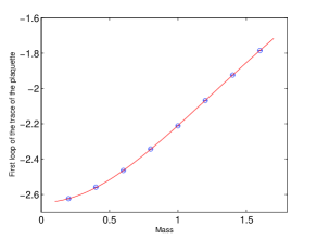
Figure 1: The 1-loop trace of the plaquette vs. mass (for $L=5$): the numerical results (blue dots) agree with the analytical red curve.

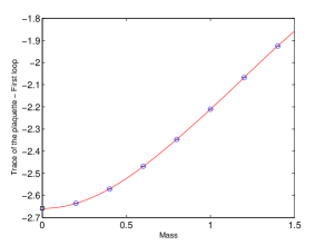
Figure 2: The 1-loop trace of the plaquette vs. mass (for $L=7$): the fitted curve in red approaches the expected value at $m=0$.

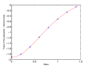
Figure 3: The 2-loop trace of the plaquette (for $L=7$), together with a polynomial fit in $m^{2}$.

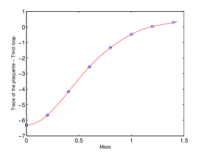
Figure 4: The 3-loop trace of the plaquette (for $L=7$), together with a polynomial fit in $m^{2}$.

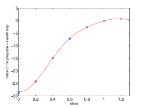
Figure 5: The 4-loop trace of the plaquette (for $L=7$), together with a polynomial fit in $m^{2}$.

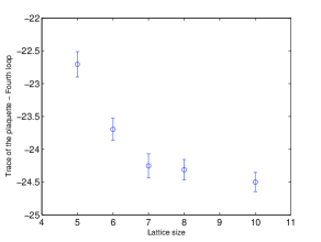
Figure 6: The 4-loop trace of the plaquette vs. lattice size, for a fixed mass $m=0.2$.

5 Conclusions and prospects

It is worth stressing once again that our approach has successfully passed the reliability checks we adopted: known zero-mass limits are reproduced through an extrapolation, and the volume dependence at a fixed mass appears to disappear once the dimensionless combination $mL$, where $m$ is the mass and $L$ the lattice extent, is large enough.

In order to obtain the asymptotic large-volume value at a fixed mass, it is still necessary to collect more statistics on bigger lattices (for example, $L=12$ and 14) at least for the two or three smallest masses. Then, the fitting function should be a combination of a negative exponential and polynomials in $mL$, as explained for instance in Ref. [12].

After subtracting the logarithmic divergence from the fitted infinite-volume values, the subsequent extrapolation to zero mass does not appear to be troublesome, given that tests with lower loop orders have produced good results so far.

References

- [1] A.D. Linde, Infrared problem in thermodynamics of the Yang-Mills gas, Phys. Lett. B 96 (1980) 289.
- [2] P. Ginsparg, First and second order phase transitions in gauge theories at finite temperature, Nucl. Phys. B 170 (1980) 388; T. Appelquist and R.D. Pisarski, High-temperature Yang-Mills theories and three-dimensional Quantum Chromodynamics, Phys. Rev. D 23 (1981) 2305.
- [3] K. Kajantie, M. Laine, K. Rummukainen and M. Shaposhnikov, Generic rules for high temperature dimensional reduction and their application to the Standard Model, Nucl. Phys. B 458 (1996) 90 [hep-ph/9508379].
- [4] E. Braaten and A. Nieto, Free energy of QCD at high temperature, Phys. Rev. D 53 (1996) 3421 [hep-ph/9510408].
- [5] G. Parisi and Y. Wu, Perturbation Theory Without Gauge Fixing, Sci. Sin. 24 (1981) 483.
- [6] F. Di Renzo, E. Onofri, G. Marchesini and P. Marenzoni, Four loop result in SU(3) lattice gauge theory by a stochastic method: Lattice correction to the condensate, Nucl. Phys. B 426 (1994) 675 [hep-lat/9405019].
- [7] F. Di Renzo, A. Mantovi, V. Miccio and Y. Schröder, 3-d lattice Yang-Mills free energy to four loops, JHEP 05 (2004) 006 [hep-lat/0404003].
- [8] A. Hietanen, K. Kajantie, M. Laine, K. Rummukainen and Y. Schröder, Plaquette expectation value and gluon condensate in three dimensions, JHEP 01 (2005) 013 [hep-lat/0412008].
- [9] K. Kajantie, M. Laine, K. Rummukainen and Y. Schröder, The pressure of hot QCD up to , Phys. Rev. D 67 (2003) 105008 [hep-ph/0211321]; Y. Schröder, Tackling the infrared problem of thermal QCD, Nucl. Phys. B (Proc. Suppl.) 129 (2004) 572 [hep-lat/0309112].
- [10] H.J. Rothe, Lattice gauge theories: An Introduction, World Sci. Lect. Notes Phys. 74 (2005) 1.
- [11] F. Di Renzo and L. Scorzato, Fermionic loops in numerical stochastic perturbation theory, Nucl. Phys. B (Proc. Suppl.) 94 (2001) 567 [hep-lat/0010064].
- [12] I. Montvay and G. Münster, Quantum fields on a lattice (Cambridge University Press, Cambridge, 1994).