A toy model of (grand) unified monopoles

Abstract:

We explore the old idea that, in a theory containing several gauge groups, the topological defects of one gauge group coincide with those of another gauge group. This simple ’unification’ constraint has deep consequences, the best known of which is a natural explanation of the fractional electric charge of quarks. Here we explore the consequences of this idea for the phase diagram, in a toy model $U(1)\times U(1)$.

PoS(LAT2005)314

1 Introduction

A while ago we measured in pure $SU(2)$ gauge theory the temperature behaviour of the free energy of various types of center vortices. Using ’t Hooft’s twisted b.c.’s we studied ratios of partition functions with an odd number of center vortices piercing the various planes of a 4-dimensional Euclidean $1/T\!\times\!L^{3}$ box relative to the periodic ensemble. Qualitatively, at low temperatures, center vortices can spread to lower their free energy. Their proliferation disorders the Wilson loop and leads to confinement. As the temperature is increased vortices through the temporal $1/T\!\times\!L$ planes are squeezed more and more. They can no-longer spread arbitrarily and this is what drives the phase transition. In the thermodynamic limit, their free energy approaches zero (infinity) for $T$ below (above) $T_{c}$ [1, 2, 3]. In the high temperature phase, macroscopic regions of Polyakov loops of a definite center sector appear, which are separated by interfaces whose tension suppresses these types of vortices leading to a dual area law for the spatial ’t Hooft loops in the high temperature phase [4]. A Kramers–Wannier duality is observed nicely in comparing the behaviour of these vortices with that of the electric fluxes which yield free energies of static charges in a well-defined (UV-regular) way [5], with boundary conditions to mimic the presence of ’mirror’ (anti)charges in neighbouring boxes. This duality follows that between the Wilson loops of the 3d $\mbox{\sf Z\mbox{}Z}_{2}$-gauge theory (the universal partners of the spatial ’t Hooft loops in $SU(2)$) and the 3d-Ising spins, reflecting the different realisations of the 3-dimensional electric center symmetry in both phases. Universality is seen at work in an impressively large scaling window around criticality [2, 6]. While the electric (fluxes)twists provide well-defined (dis)order parameters for confinement, the free energy of the magnetic ones vanishes exponentially at all $T$ in the thermodynamic limit. The corresponding screening of temporal ’t Hooft loops is determined by the spatial string tension, and center monopoles always ’condense’ [7]. Combinations of electric and magnetic twists can however be used to measure the topological susceptibility without cooling [8].

While the techniques can be extended to compute interface tensions for $SU(N)$ with $N\geq 3$ and phase coexistence [9], the nagging question remains as to what the significance is of these qualitatively and quantitatively quite compelling results when dynamical quarks with their fundamental charges are included. Even in presence of quite heavy dynamical quarks the picture becomes rather murky. Upon encircling an interface (which is a line-defect in 3 dimensions) they pick up a non-trivial phase corresponding to their fundamental charge. This multivaluedness thus seems to have a dramatic effect on the dynamics of the same topological defects that appear to describe the phases of the pure gauge theory so beautifully. Should it be true that the phase structure changes abruptly when going from infinitely heavy to no-matter-how-large but finite quark masses? At least it would seem rather unnatural to assume that there are entirely different mechanisms in either case, which nevertheless lead to a smooth limit.

In the next section we briefly discuss a tantalising possibility for the coexistence of quarks and interfaces by simple unification constraints in theories with several gauge groups as in $SU(3)\times U(1)$. In Section 3 we explore this same idea in a toy model $U(1)\times U(1)$. The considerable consequences of defect unification as exemplified in the toy model are discussed in our conclusions. The idea of unification constraints for topological defects, which might arise quite naturally from grand unified theories, with topological defects such as e.g. the $SU(5)$ monopole [10], is not new but certainly deserves renewed interest and further study.

2 Quarks and Interfaces

The problem with quarks and interfaces arises because a center-vortex sheet, which can be moved freely in the pure gauge ensemble, now becomes observable. Technically, with fundamental fields there are no twisted boundary conditions to measure vortex free energies in the first place. One way out of this dilemma might be provided by combining $SU(3)$ with $U(1)$ defects, realising that quarks have fractional electric charges and interact with both gluons and photons. As pointed out by Creutz in his last year’s Lattice proceedings [11], there is a remarkable phase cancellation when quarks encircle a combined $\mbox{\sf Z\mbox{}Z}_{3}$ and Dirac string. This is due to their fractional electric charges and makes such combined strings unobservable.

In particular, upon encircling a $\mbox{\sf Z\mbox{}Z}_{3}$ string, quarks pick up phases of $e^{i2\pi/3}$ or $e^{i4\pi/3}$ depending on the kind of string (i.e. interface in 4d). On the other hand, depending on their fractional electric charges, $2/3$ or $-1/3$ in units of $e$, these two phases can add to produce multiples of $2\pi$ for the combined string. In particular, independently of the quark’s flavour this phase cancellation happens for the first type of $\mbox{\sf Z\mbox{}Z}_{3}$ string whenever the accompanying Dirac flux is $m=1\textrm{ mod }3$ (in units of $2\pi/e$), while for the second it requires $m=-1\textrm{ mod }3$ (one easily verifies that all other combinations lead to non-integer fractions of $2\pi$ for the total phases of quarks with either charge).

Thus, if we combine in this way $SU(3)$ ’t Hooft with $U(1)$ monopole loops, and the respective center-vortex/Dirac sheets spanned by the two, the dynamics of the so combined defects might allow to smoothly connect quark confinement to that of static fundamental charges in the pure gauge theory. Of course, the defect-unification constraint induces a coupling between the two gauge groups. The dynamics of the formation/suppression of one kind of defect is now tied to the other. We will explore this effect in a toy model.

3 Toy Model

Consider the 4d compact pure Abelian gauge theory with Wilson action for the gauge group $U(1)\times U(1)$,

$$S\,=\,-\beta_{1}\sum_{P}\cos\theta_{P}^{(1)}-\beta_{2}\sum_{P}\cos\theta_{P}^{(2)}\;,$$ (1)

with two couplings $\beta_{i}=1/e_{i}^{2}$ and plaquette angles $\theta^{(i)}_{P}$, $i=1,2$. Without any constraints the phases are trivially determined by the 2 independent $U(1)$ factors. The phase transitions at $\beta_{c}$ just above 1 can be seen in the monopole densities, the string tension and the helicity modulus [12] yielding the phase diagram as sketched in Fig. 1. Especially the (temporal) helicity modulus has recently reemerged as a suitable and convenient order parameter for compact $U(1)$ [13]. It measures the susceptibility of the theory to static external fluxes and plays a role analogous to that of fluxes by twisted boundary conditions, albeit being more easily amenable to simulations.

                                                                

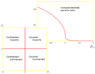
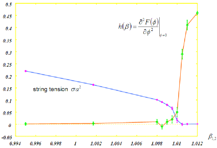
Figure 1: Without constraint the monopole density (upper left), string tension and helicity modulus (right) of 4d compact $U(1)$ hold for each factor implying the 4 phases in the $(\beta_{1},\beta_{2})$-plane as sketched (left).

The picture changes considerably when the two $U(1)$ factors are constrained to always have the same monopole content. This is achieved as follows: We start with identical copies of gauge field configurations for both $U(1)$’s. We then propose independent small variations for each link of the two gauge fields a la Metropolis. In addition to the usual probability by the Wilson action the monopole currents in both $U(1)$’s must however also remain the same for the updates to be accepted, though they may both be changed of course in each step (the step size is chosen to achieve an acceptance rate of about 50%). This is controlled by comparing the units of magnetic charge $m$ in the cubes sharing the updated links.

The phase diagram now changes dramatically as seen in Fig. 2. One large enough $\beta$ (small coupling) suffices to suppress the monopoles in both $U(1)$ groups, no matter how strong the second coupling is. We are left with only 2 phases, the same for both $U(1)$’s, and the mixed phases no-longer exist. The transition occurs at somewhat smaller values of $\beta$; we roughly estimate $0.39$ along the diagonal $\beta_{1}=\beta_{2}$ and $0.62$ near the axes where one of the two $\beta$’s approaches zero. A precise determination remains to do be done, however. Both string tensions (not shown here) are the same also for $\beta_{1}\not=\beta_{2}$ and vanish at the transition line in the two coupling plane. These correspond however to Wilson loops of charges $(1,0)$ and $(0,1)$ (in units of $e$).

More interesting for our purposes are the half-odd integer cases $(1/2,\pm 1/2)$ which can exist in $U(1)\times U(1)$ with monopole unification constraint because of the same phase cancellation as described in Sec. 2. Instead of a direct measurement of the corresponding Wilson loops, here we present preliminary results for the helicity moduli which mimic the response to the presence of static charges. In presence of constant (homogeneous) fluxes $\phi^{(i)}$ through a $(\mu,\nu)$-plane (of size $L_{\mu}L_{\nu}$), the action of each $U(1)$ factor is modified for all plaquettes $P(\mu,\nu)$ with $(\mu,\nu)$-orientation,

$$S_{i}(\phi^{(i)})=-\beta_{i}\mbox{}\sum_{P\in\{P(\mu,\nu)\}}\mbox{}\cos\big{(}\theta^{(i)}_{P}+\mbox{\hskip 1.99997pt}\raisebox{2.15277pt}{$\displaystyle\phi^{(i)}$}\mbox{}/\raisebox{-2.15277pt}{$\displaystyle(L_{\mu}L_{\nu})$}\big{)}-\beta_{i}\mbox{}\sum_{P\not\in\{P(\mu,\nu)\}}\mbox{}\cos\theta^{(i)}_{P}\;\;,\quad i=1,\,2\;.$$ (2)

Since the fluxes of both factors are independent, the helicity modulus defined as the curvature of the free energy at vanishing flux now has 3 independent components according to the Hessian

$$H(\beta_{1},\beta_{2})\,=\,\left(\frac{\partial^{2}F(\phi^{(1)},\phi^{(2)})}{\partial\phi^{(i)}\partial\phi^{(j)}}\bigg{|}_{0}\right)\;.$$ (3)

The diagonal components are the susceptibilities of the coupled theory to flux in one of the two $U(1)$ factors alone. Their behaviour should reflect that of the $(1,0)$ and $(0,1)$ Wilson loops. For objects equally(oppositely) charged w.r.t. both, we need the curvature of free energy in the $(1,\pm 1)$ directions corresponding to helicity moduli $h^{\pm}=H_{11}+H_{22}\pm 2H_{12}$,

$$h^{\pm}(\beta_{1},\beta_{2}) = \frac{1}{(L_{\mu}L_{\nu})^{2}}\left\{\sum_{i=1,2}\Big{(}\Big{\langle}\beta_{i}\mbox{}\sum_{P\in\{P(\mu,\nu)\}}\mbox{}\cos\theta^{(i)}_{P}\Big{\rangle}-\Big{\langle}\Big{(}\beta_{i}\mbox{}\sum_{P\in\{P(\mu,\nu)\}}\mbox{}\sin\theta^{(i)}_{P}\Big{)}^{2}\Big{\rangle}\Big{)}\right.$$

$$\hskip 113.81102pt\mp\,2\left.\Big{\langle}\Big{(}\beta_{1}\mbox{}\sum_{P\in\{P(\mu,\nu)\}}\mbox{}\sin\theta^{(1)}_{P}\Big{)}\Big{(}\beta_{2}\mbox{}\sum_{P\in\{P(\mu,\nu)\}}\mbox{}\sin\theta^{(2)}_{P})\Big{)}\Big{\rangle}\right\}\;.$$

Near the transition line we observe a drop of about 50% for the helicity modulus in $(1,0)$, $(0,1)$, i.e. for flux in just one of the $U(1)$’s. Contrary to the unconstrained case, however, it does not drop to zero on the strong coupling side as seen for $\beta_{1}=\beta_{2}$ in Fig. 3. Our preliminary data on $h^{\pm}(\beta_{1},\beta_{2})$ indicates, however, that this is due to the very different behaviour of equal versus opposite fluxes. Presumably, fields with equal electric charges in both $U(1)$’s are confined by the condensation of the unified monopoles, while oppositely charged ones are not. This would open further interesting possibilities. One might ask for instance, what happens if we relax the constraint to include oppositely charged $\pm m$ magnetic monopoles sitting on top of each other? Would that confine the opposite electric charges together with the equal ones?

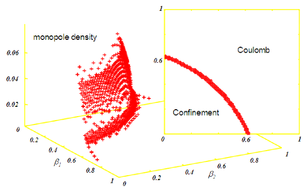
Figure 2: Monopole density (relative number of cubes with $m\!\not=0$) and transition line estimate in the 2 coupling plane of $U(1)\times U(1)$ with monopole unification constraint (on a $12^{4}$ lattice). The relatively small probability of having a monopole in any given cube is further reduced in the constrained case, and the transition to the confined phase is thus shifted towards the origin in the $(\beta_{1},\beta_{2})$-plane.

4 Conclusions

Our toy model serves to demonstrate that in theories with several gauge groups it can be deceiving to study the individual factors separately, especially when there are mechanisms by which the defects of one gauge group are forced to coincide with those of another. Such unification constraints have been suggested to arise naturally from grand unified theories and might manifest themselves in the presence of fundamental fields such as quarks in QCD or other particles with fractional charges in several gauge groups. It appears to be worthwhile to explore the idea of defect unification in other models such as a double Abelian Higgs model with fractional charges, or revisit $SU(2)\times U(1)$ with fundamental Higgs fields in the light of defect-unification constraints.

Another interesting property of the toy model $U(1)\times U(1)$ is its capacity to confine equal charge doublets whereas oppositely charged ones do not see the unified monopoles but only the topologically trivial gauge field fluctuations, and thus retain a Coulomb-like behaviour at any coupling. At least, our preliminary data on the corresponding helicity moduli is fully consistent with what one expects for such a behaviour. A more quantitative analysis is under way.

Finally, and maybe most importantly, however, one should probably address such questions as: What kind of constraints can we get from defects in grand unified theories, and what do we need to confine quarks but not electrons?

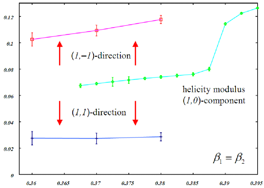
Figure 3: Susceptibility to flux in one of the two $U(1)$ factors with monopole-unification for $\beta_{1}=\beta_{2}$ (on a $12^{4}$ lattice). Preliminary data for equal and opposite fluxes (the helicity moduli in $(1,\pm 1)$ directions) in the strong coupling regime are also shown indicating a level splitting. A precise analysis, a study of their transition behaviour and of finite-size effects are yet to be done. However, this is a first sign of the different behaviour of states with equal and opposite charges in both gauge groups (which may each be half-odd integer).

References

- [1] T. G. Kovacs and E. T. Tomboulis, Phys. Rev. Lett. 85 (2000) 704 [hep-lat/0002004].
- [2] L. von Smekal, with Ph. de Forcrand, in Confinement, Topology and other Non-Perturbative Aspects of QCD, Eds. J. Greensite and Š. Olejník, NATO Sci. Ser., Kluwer (2002) 287 [hep-ph/0205002].
- [3] Ph. de Forcrand and L. von Smekal, Phys. Rev. D66 (RC) (2002) 011504 [hep-lat/0107018].
- [4] Ph. de Forcrand, M. D’Elia and M. Pepe, Phys. Rev. Lett. 86 (2001) 1438 [hep-lat/0007034].
- [5] Ph. de Forcrand and L. von Smekal, Nucl. Phys. (PS) B106 (2002) 619 [hep-lat/0110135].
- [6] M. Pepe and Ph. de Forcrand, Nucl. Phys. (PS) 106 (2002) 914 [hep-lat/0110119].
- [7] L. von Smekal, with Ph. de Forcrand, Nucl. Phys. (PS) B119 (2003) 655 [hep-lat/0209149].
- [8] L. von Smekal, with Ph. de Forcrand and O. Jahn, in Quark Confinement and the Hadron Spectrum V, Eds. N. Brambilla and G. M. Prosperi, World Scientific (2003) 303 [hep-lat/0212019].
- [9] Ph. de Forcrand, B. Lucini and M. Vettorazzo, Nucl. Phys. (PS) B140 (2005) 647 [hep-lat/0409148].
- [10] M. Srednicki and L. Susskind, Nucl. Phys. B179 (1981) 239.
- [11] M. Creutz, Nucl. Phys. (PS) B140 (2005) 597 [hep-lat/0408013].
- [12] M. Vettorazzo and Ph. de Forcrand, Nucl. Phys. B686 (2004) 88 [hep-lat/0311006].
- [13] M. Vettorazzo and Ph. de Forcrand, Phys. Lett. B604 (2004) 82 [hep-lat/0409135].