Dirac-Kähler fermions and exact lattice supersymmetry

Abstract:

We discuss a new approach to putting supersymmetric theories on the lattice. The basic idea is to start from a twisted formulation of the underlying supersymmetric theory in which the fermions are represented as grassmann valued antisymmetric tensor fields. The original supersymmetry algebra is replaced by a twisted algebra which contains a scalar nilpotent supercharge $Q$. Furthermore the action of the theory can then be written as the $Q$-variation of some function. The case of ${\cal N}=2$ super Yang-Mills theory in two dimensions is discussed in some detail. We then present our proposal for discretizing this theory and derive the resultant lattice action. The latter is local, free of spectrum doubling, gauge invariant and preserves the scalar supercharge invariance exactly. Some preliminary numerical results are then presented. The approach can be naturally generalized to yield a lattice action for ${\cal N}=4$ super Yang-Mills in four dimensions.

PoS(LAT2005)006

1 Introduction

Supersymmetric field theories exhibit many remarkable properties. Chief among these are the cancellations which occur between boson and fermion contributions in the perturbative calculation of physical quantities. These cancellations eliminate many of the divergences typical of quantum field theory and are at the heart of its use to solve the gauge hierarchy problem [1]. Additionally, supersymmetric versions of Yang Mills theory, while more tractable analytically than their non-supersymmetric counterparts, exhibit many of the same features such as confinement and chiral symmetry breaking [2]. Super Yang-Mills theories with extended supersymmetry are also conjectured to be dual to various supergravity theories in the limit of a large number of colors and have been proposed as a regularization for M-theory [3, 4].

Since low energy physics is manifestly not supersymmetric it is necessary that this symmetry be broken at some energy scale. A set of non-renormalization theorems ensure that if SUSY is not broken at tree level then it cannot be broken in any finite order of perturbation theory see eg. [1]. Thus the general expectation is that any breaking should occur non-perturbatively. The lattice furnishes the only tool for a systematic investigation of non-perturbative effects in field theories and so significant effort has gone into formulating SUSY theories on the lattice – see [5] and the recent reviews [6],[7].

Unfortunately, there are several barriers to such lattice formulations. Firstly, supersymmetry is a spacetime symmetry which is generically broken by the discretization procedure. In this it resembles Poincare invariance which is also not preserved in a lattice theory. However, unlike Poincare invariance there is usually no SUSY analog of the discrete translation and cubic rotation groups which are left unbroken on the lattice. In the latter case the existence of these remaining discrete symmetries is sufficient to prohibit the appearance of relevant operators in the long wavelength lattice effective action which violate the full symmetry group. This ensures that Poincare invariance is achieved automatically without fine tuning in the continuum limit. Since generic latticizations of supersymmetric theories do not have this property their effective actions typically contain relevant supersymmetry breaking interactions. To achieve a supersymmetric continuum limit then requires fine tuning the bare lattice couplings of all these SUSY violating terms - typically a very difficult proposition.

Secondly, supersymmetric theories necessarily involve fermionic fields which generically suffer from doubling problems when we attempt to define them on the lattice. The presence of extra fermionic modes furnishes yet another source of supersymmetry breaking since typically they are not paired with corresponding bosonic states. Furthermore, most methods of eliminating the extra fermionic modes serve to break supersymmetry also.

Recently there has been renewed interest in this problem stemming from the realization that in certain classes of theory it may be possible to preserve at least some of the supersymmetry exactly at finite lattice spacing. It is hoped that this residual supersymmetry may protect the lattice theory from the dangerous SUSY-violating radiative corrections that leading to fine tuning. In the case of extended supersymmetry two approaches have been followed; in the first, pioneered by Kaplan and collaborators, the lattice theory is constructed by orbifolding a certain supersymmetric matrix model and then extracting the lattice theory by expansion around some vacuum state [10, 11, 12, 13]. The second approach relies on reformulating the supersymmetric theory in terms of a new set of variables – the twisted fields. In this procedure a scalar nilpotent supercharge is exposed and it is the algebra of this charge that one may hope to preserve under discretization [14],[15], [16]. This approach was initially used to construct and study lattice formulations of a variety of low dimensional theories without gauge symmetry [17, 18, 19, 20, 21]. Subsequently it was extended to case of Yang-Mills theories by Sugino [22, 23] although that construction was confined to low dimensional theories. In this review we will confine ourselves to a discussion of a new geometrical discretization of the twisted theory which accommodates both two and four dimensional super Yang Mills theories.

The basic idea in this approach is decompose the fermion fields as a set of antisymmetric tensor fields which are subsequently interpreted as components of single Dirac-Kähler field. This same procedure when applied to the supercharges exposes a scalar nilpotent supercharge $Q$. Furthermore, the action of the supersymmetric field theory can then be written as the $Q$-variation of some function. Provided we can then maintain the nilpotent property of $Q$ under discretization it is straightforward to write down a lattice action in terms of these twisted fields which is exactly invariant under $Q$ at finite lattice spacing. As a bonus we will find that that this twisted formulation of the theory, being written entirely in geometrical terms, can be discretized without encountering spectrum doubling.

We first describe the nature of the twist in two dimensions and explain how it is related to the use of Dirac-Kähler fermions. We then give a detailed discussion of continuum ${\cal N}=2$ super Yang-Mills in two dimensions which furnishes a simple example of the twisted approach. Our discretization prescription is then introduced and a lattice action for this theory constructed. The latter is local, free of spectrum doubling, gauge invariant and preserves a single (twisted) supersymmetry at finite lattice spacing. It is naturally formulated in terms of complex fields and we discuss how this lattice model may be used to target the true continuum theory. Preliminary results are then shown coming from a RHMC simulation of this lattice model which indeed show an exact $Q$-symmetry emerging at large coupling $\beta$. The technique can be generalized to provide a lattice action for ${\cal N}=4$ super Yang-Mills in four dimensions and this is then discussed in some detail.

2 The 2D Twist

Consider a theory with ${\cal N}=2$ supersymmetry in two dimensional Euclidean space. Such a theory contains two Majorana supercharges $q^{I}_{\alpha}$ transforming under the global symmetry group $SO(2)\times SO_{R}(2)$ where the subscript corresponds to two dimensional rotations and the superscript describes the behavior under the R-symmetry corresponding to rotating the two Majorana fields into one another.

The basic idea of twisting which goes back to Witten [24] is to introduce a new rotation group

$$SO(2)^{\prime}={\rm diagonal\;subgroup}(SO(2)\times SO(2)_{R})$$ (1)

and to decompose all fields now as representations of this new rotation group. In simple terms what this means is that whenever I do a rotation in the base space by some angle I must do an equal rotation in the R-symmetry space. Thus it is equivalent to treating the two indices $I$ and $\alpha$ as equivalent. Thus the supercharges are to be interpreted as matrices in this twisted picture [25, 26, 16, 27].

$$q^{I}_{\alpha}\to q_{\alpha\beta}$$ (2)

It is now natural to expand such a matrix on a basis of products of 2D gamma matrices

$$q=QI+Q_{\mu}\gamma_{\mu}+Q_{12}\gamma_{1}\gamma_{2}$$ (3)

The fields $(Q,Q_{\mu},Q_{12})$ are called the twisted supercharges. The original SUSY algebra then implies a corresponding twisted algebra which takes the form

$$\{q,q\}_{\alpha\beta}=4\gamma^{\mu}_{\alpha\beta}p^{\mu}$$ (4)

In components this reads

$$\{Q,Q\} = \{Q_{12},Q_{12}\}=\{Q,Q_{12}\}=\{Q_{\mu},Q_{\nu}\}=0$$ (5)

$$\{Q,Q_{\mu}\} = P_{\mu}$$ (6)

$$\{Q_{12},Q_{\mu}\} = -\epsilon_{\mu\nu}P_{\nu}$$ (7)

Notice that the scalar component of the supercharge matrix is nilpotent as previously advertised. It is also important to realize that the twisted superalgebra implies that the momentum $P$ is now the $Q$-variation of something – it is said to be $Q$-exact. This fact renders it plausible that the entire energy momentum tensor may be $Q$-exact in such twisted theories. Since $T_{\mu\nu}=\frac{\delta S}{\delta g_{\mu\nu}}$ this would imply that the entire action of the theory could be written in a $Q$-exact form $S=Q\Lambda$ [27]. This turns out to be true in essentially all the theories that have been studied. Specifically we will show that the action of ${\cal N}=2$ super Yang-Mills theory in two dimensions can be written in this way [28]. Notice also that to match the four real supercharges of the original supersymmetric theory it is natural to take the twisted supercharges to be real also. This in turn implies that the supercharge matrix obeys a reality condition

$$\overline{q}=q^{\dagger}=q^{T}\;{\rm in\;2D}$$ (8)

If the presence of a nilpotent scalar fermionic charge and a corresponding $Q$-exact action all sound reminiscent of BRST gauge fixing you would be right. These twisted theories can be derived by gauge fixing an underlying topological symmetry [29]. If the gauge fixing function is chosen carefully the resultant theory can be untwisted to reveal an associated supersymmetric field theory. However, it must be stressed that this correspondence is not one to one. In the topological field theory the set of physical states must be restricted in the usual way to those annihilated by the scalar charge. In the language of the supersymmetric field theory such a constraint would project one to the vacuum state. This explains why such a theory contains no physically propagating degrees of freedom – it is a theory defined only on the moduli space of classical solutions. Our proposal is not to impose this physical state condition but merely to treat the twisting procedure as an exotic change of variables in the supersymmetric field theory. Certainly in flat space the physical content of the twisted and untwisted theories is the same.

Let us turn now to a discussion of the fields in such a twisted theory. It should be clear that if the supercharges can be written as matrix so can the fermions

$$\Psi=\frac{\eta}{2}I+\psi_{\mu}\gamma_{\mu}+\chi_{12}\gamma_{1}\gamma_{2}$$ (9)

Thus the twisted theory will not contain spinors but antisymmetric tensor fields. Indeed it is possible to abstract these p-form fields and consider them as components of a geometrical object – a Dirac-Kähler field as first emphasized by Kawamoto and collaborators [16].

$$\Psi=(\frac{\eta}{2},\psi_{\mu},\chi_{12})$$ (10)

It is a remarkable fact that the original Dirac equation for 2 (Majorana) fermions is then equivalent to the geometrical Dirac-Kähler equation [30]

$$(d-d^{\dagger})\Psi=0$$ (11)

Here $d$ and $d^{\dagger}$ are the usual exterior derivative and its adjoint. Their action on a generic Dirac-Kähler field $\omega$ is given by

$$d\omega=\left(0,\partial_{\mu}f,\partial_{\mu}f_{\nu}-\partial_{\nu}f_{\mu},\ldots\right)$$ (12)

and

$$-d^{\dagger}\omega=\left(f^{\nu},f^{\nu}_{\mu},\ldots,0\right)_{;\nu}$$ (13)

The Dirac-Kähler equation can be derived from an action

$$S_{F}=\left<\Psi^{\dagger}.(d-d^{\dagger})\Psi\right>$$ (14)

where the dot product of two Dirac-Kähler fields $A$ and $B$ is defined by

$$<A|B>=\int d^{D}x\sqrt{g}\sum_{p}\frac{1}{p!}A^{\mu_{1}\ldots\mu_{p}}B_{\mu_{1}\ldots\mu_{p}}$$ (15)

Writing out these components explicitly and restricting ourselves to flat space we find

$$S_{F}=\frac{1}{2}\psi^{\dagger}_{\mu}\partial_{\mu}\eta+\frac{1}{2}\chi^{\dagger}_{\mu\nu}\partial_{\left[\mu\right.}\psi_{\left.\nu\right]}$$ (16)

This equivalence of the Dirac equation to the Dirac-Kähler equation holds equally when ordinary derivatives are replaced by gauge covariant derivatives.

The usual reason why the Dirac equation is preferred over the Dirac-Kähler equation is that the latter naturally describes the propagation of 2 degenerate fermions in two dimensions. In a theory like QCD where the bare quark masses are not usually thought of as equal this appears problematic. However, a theory with ${\cal N}=2$ supersymmetry in $D=2$ dimensions naturally requires such degenerate fermionic states. Thus we have argued that for these special theories the twisting procedure we have described is actually exactly equivalent to the decomposition of the fermion fields in terms a single Dirac-Kähler field. Furthermore the equivalence between the Dirac equation and the Dirac-Kähler equation holds also in four dimensions where the latter equations describes the propagation of four degenerate (Majorana) fermions. Again, this is precisely the field content of ${\cal N}=4$ super Yang-Mills theory and we should not be surprised then to find out that the latter theory when suitably twisted can be expressed in terms of the components of a single real Dirac-Kähler field [31],[32].

Finally any theory invariant under the $Q$-symmetry must contain superpartners for these fermionic fields. In two dimensions we then expect to find the following bosonic (commuting) fields

$$(\overline{\phi},A_{\mu},B_{12})$$ (17)

The nilpotency of $Q$ then requires that $Q^{2}=0$ up to gauge transformations when acting on any of these component fields. If we interpret $B_{12}$ as a multiplier field we see that in this way we have generated the bosonic field content of ${\cal N}=2$ SYM in 2D if we interpret each field as taking values in the adjoint of some gauge group. We turn now to an explicit construction of the twisted form of this theory.

3 Twisted ${\cal N}=2$ SYM in $D=2$

In this section we render all these ideas concrete by writing down the twisted formulation of ${\cal N}=2$ super Yang-Mills theory in two (continuum) dimensions. The construction will expose the scalar supersymmetric invariance explicitly and the $Q$-exact form of the action. We will also show that the resulting on-shell action can be rewritten in terms of the usual spinor degrees of freedom exhibiting the fact that (in flat space) the twisted theory is nothing but a change of variables in the original spinor based super Yang-Mills model. The twisted gauge fermion is written [28],[22]

$$S = \beta Q{\rm Tr}\int d^{2}x\left(\frac{1}{4}\eta[\phi,\overline{\phi}]+2\chi_{12}F_{12}+\right.$$ (18)

$$+ \left.\chi_{12}B_{12}+\psi_{\mu}D_{\mu}\overline{\phi}\right)$$ (19)

where each field is in the adjoint of some gauge $U(N)$ group $X=\sum_{a=1}^{N}X^{a}T^{a}$ and we employ antihermitian generators $T^{a}$. The action of $Q$ on the fields is given by

$$QA_{\mu} = \psi_{\mu}$$

$$Q\psi_{\mu} = -D_{\mu}\phi$$

$$Q\phi = 0$$

$$Q\chi_{12} = B_{12}$$

$$QB_{12} = [\phi,\chi_{12}]$$

$$Q\overline{\phi} = \eta$$

$$Q\eta = [\phi,\overline{\phi}]$$ (20)

Notice that $Q^{2}$ generates an (infinitessimal) gauge transformation parametrized by the field $\phi$. Carrying out the $Q$-variation and subsequently integrating out the multiplier field $B_{12}$ we find the on-shell action

$$S = \beta{\rm Tr}\int d^{2}x\left(\frac{1}{4}[\phi,\overline{\phi}]^{2}-\frac{1}{4}\eta[\phi,\eta]-F_{12}^{2}\right.$$ (21)

$$- D_{\mu}\phi D_{\mu}\overline{\phi}-\chi_{12}[\phi,\chi_{12}]$$ (22)

$$- 2\chi_{12}\left(D_{1}\psi_{2}-D_{2}\psi_{1}\right)-2\psi_{\mu}D_{\mu}\eta/2$$ (23)

$$+ \left.\psi_{\mu}[\overline{\phi},\psi_{\mu}]\right)$$ (24)

The gauge and scalar part of this action are easily recognized to be the usual bosonic sector of ${\cal N}=2$ super Yang-Mills. If I choose the contour where $\overline{\phi}^{a}=(\phi^{a})^{*}$ it is clear that the bosonic action is real and positive semi-definite. The fermionic sector looks a little unconventional but by looking back at the previous discussion it can be seen that it merely corresponds to a Dirac-Kähler decomposition of the usual spinor action corresponding to two Majorana fermions. To convince ourselves of the equivalence of this twisted formulation to the usual one it is convenient to pick a Euclidean chiral basis for the two dimensional $\gamma$-matrices

$$\begin{array}[]{cc}\gamma_{1}=\left(\begin{array}[]{cc}0&1\\ 1&0\end{array}\right)&\gamma_{2}=\left(\begin{array}[]{cc}0&i\\ -i&0\end{array}\right)\end{array}$$ (25)

and to subsequently define a Dirac spinor $\lambda$ as

$$\lambda=\left(\begin{array}[]{c}\frac{\eta}{2}-i\chi_{12}\\ \psi_{1}-i\psi_{2}\end{array}\right)$$ (26)

It is then a straightforward exercise to show that the Dirac action $\lambda^{\dagger}\gamma.D\lambda$ reduces to the kinetic terms in the twisted action we have previously uncovered. Indeed the entire twisted action including the Yukawas can be rewritten in terms of this Dirac spinor and can be recognized as the usual fermionic sector of two dimensional ${\cal N}=2$ super Yang-Mills.

$$S=\lambda^{\dagger}M(\phi)\lambda$$ (27)

where

$$M=\gamma.D+\frac{\left(1+\gamma_{5}\right)}{2}[\overline{\phi},\cdots]-\frac{\left(1-\gamma_{5}\right)}{2}[\phi,\cdots]$$ (28)

4 Discretization

We will adopt this geometrical formulation as a useful starting off point for constructing a lattice theory. It is convenient from the point of view of supersymmetry as the scalar component of the twisted supersymmetry involves no derivatives and offers the hope, therefore, of being compatible with a lattice structure. Secondly, the use of Dirac-Kähler fermions is attractive as it is known how to discretize the Dirac-Kähler action without inducing spectrum doubling. Indeed, Dirac-Kähler fermions at the level of free field theory are known to be equivalent to staggered fermions. The usual degeneracy of staggered fermions now becomes a plus – it allows us to replicated the degenerate flavors required by extended supersymmetry. The use of Dirac-Kähler fermions to formulate (Hamiltonian) lattice supersymmetric models was first proposed in [33].

Clearly, continuum scalar fields should map to fields defined on sites in a (hypercubic) lattice, continuum vector fields to fields defined on links and rank 2 antisymmetric fields to lattice fields living on plaquettes. Notice that all lattice p-cubes whose dimension is greater than zero come in two possible orientations corresponding to whether the defining vertices are written down as an even or odd permutation of some standard ordering. In the case of links this is just the usual statement that the link has two possible directions. It is then natural (and as we will see later essential) that this 2-fold orientation of the underlying p-cube can be associated with the existence of two independent lattice fields for each continuum field. These two fields can be represented by allowing the lattice fields $X^{a}$ to be complex numbers thus promoting the group from $U(N)$ to $GL(N,C)$. The lattice fields are also assigned gauge transformation properties which generalize the usual transformation properties of site fields and links in lattice gauge theory [34]:

$$f(x) \to G(x)f_{(}x)G^{-1}(x)$$ (29)

$$f_{\mu}(x) \to G(x)f_{\mu}(x)G^{-1}(x+\mu)$$ (30)

$$f_{12}(x) \to G(x)f_{12}(x)G^{-1}(x+1+2)$$ (31)

where $G=e^{\phi}$ is a lattice gauge transformation. Notice in the naive continuum limit where $G\sim 1+\phi$ these reduce to the usual commutator structure typical of adjoint fields. In general this leads to a point split or shifted commutator. For link fields this looks like

$$[\phi(x)f_{\mu}(x)-f_{\mu}(x)\phi(x+\mu)]$$ (32)

Notice that this commutator has a well-defined lattice gauge transformation property. Finally, we must replace the continuum gauge connection $A_{\mu}$ with a Wilson gauge link $U_{\mu}(x)=e^{A_{\mu}}$. Notice now that $A_{\mu}$ will be complex which implies that the gauge links are not unitary at this stage in the construction.

Of course we have not yet finished. We need also to give a prescription for replacing continuum covariant derivatives by difference operators. Furthermore, as we will argue later, we are naturally led to use covariant versions of forward and backward difference operators. The results of these difference operators when acting on lattice fields should also result in new lattice fields with well-defined gauge transformation properties. Thus hitting a site field with such a (forward) difference operator should lead to a field which gauge transforms like a link field etc. It is not hard to show that the following definition of a forward difference operator acting on site and link field satisfy these properties [34]

$$D^{+}_{\mu}f(x) = U_{\mu}(x)f(x+\mu)-f(x)U_{\mu}(x)$$ (33)

$$D^{+}_{\mu}f_{\nu}(x) = U_{\mu}(x)f_{\nu}(x+\mu)-f_{\nu}(x)U_{\mu}(x+\nu)$$ (34)

They clearly reduce to continuum derivatives as $a\to 0$ and ensure that the resulting fields gauge transform in the appropriate way. Rather remarkably it is possible to write a covariant backward difference which is truly adjoint to the above operator for gauge invariant quantities. Notice that it will necessarily act as a divergence operation (for a proof of this statement we refer the reader to the paper by Aratyn et al [34])

$$D^{-}_{\mu}f_{\mu}(x) = f_{\mu}(x)U^{\dagger}_{\mu}(x)-U^{\dagger}_{\mu}(x-\mu)f_{\mu}(x-\mu)$$ (35)

$$D^{-}_{\mu}f_{\mu\nu}(x) = f_{\mu\nu}(x)U^{\dagger}_{\mu}(x+\nu)-U^{\dagger}_{\mu}(x-\mu)f_{\mu\nu}(x-\mu)$$ (36)

We have now almost all the ingredients needed to construct our lattice super Yang-Mills theory. The remaining key observation goes back to work by Becher, Joos, Rabin and others [35, 36] concerning discretizing actions written in terms of p-forms and exterior derivatives. They give a topological proof using results from homology theory that such actions can be discretized in such a way that the resulting lattice theories are completely free of spectrum doubling – that is, the resulting lattice theories do not contain any modes having no analog in the continuum theory. However, such theories, like staggered fermion models, will necessarily describe degenerate flavors of fermion. While this is a problem for QCD it is a bonus in the supersymmetric theories studied here as these degenerate flavors can represent the multiple fermions inherent in extended supersymmetry. While these original papers showed how to do this for ordinary derivatives, a generalization to covariant derivatives was first given by Aratyn at al.[34] which is the one employed here. The discretization prescription is given explicitly by replacing the usual partial derivatives in the continuum theory by appropriate difference operators:

$D_{\mu}\to D^{+}$ if it acts like $d$

$D_{\mu}\to D^{-}$ if it acts like $d^{\dagger}$

Following this rule we find that the Yang-Mills field strength is discretized as follows

$$F_{\mu\nu}(x)=D^{+}_{\mu}U_{\nu}(x)\to F^{\rm cont}_{\mu\nu}\;{\rm as}\;a\to 0$$ (37)

Notice it is automatically antisymmetric in its indices. Using these ingredients we propose the following lattice action for ${\cal N}=2$ super Yang-Mills

$$S_{L} = \frac{1}{2}\beta Q{\rm Tr}\sum_{x}\left(-\frac{1}{4}\eta^{\dagger}[\phi,\overline{\phi}]-2\chi^{\dagger}_{12}F_{12}\right.$$ (38)

$$- \left.\chi^{\dagger}_{12}B_{12}-\psi^{\dagger}_{\mu}D^{+}_{\mu}\overline{\phi}+{\rm h.c}\right)$$ (39)

Notice the necessity of introducing both fields and their hermitian conjugates in order to write down gauge invariant expressions. The corresponding lattice supersymmetry is a simple generalization of the continuum ones [28]

$$QU_{\mu} = \psi_{\mu}$$

$$Q\psi_{\mu} = -D^{+}_{\mu}\phi$$

$$Q\phi = 0$$

$$Q\chi_{12} = B_{12}$$

$$QB_{12} = [\phi,\chi_{12}]^{(12)}$$

$$Q\overline{\phi} = \eta$$

$$Q\eta = [\phi,\overline{\phi}]$$ (40)

where I have replaced $D_{\mu}\phi$ by $D^{+}_{\mu}\phi$ as required by gauge invariance and the prime reflects the fact that we must use a shifted commutator as previously discussed. Carrying out the $Q$-variation and then integrating out the field $B$ as in the continuum we obtain the on-shell lattice action

$$S_{L} = \frac{\beta}{2}{\rm Tr}\sum_{x}\left(\frac{1}{4}[\phi,\overline{\phi}]^{2}+F^{\dagger}_{12}F_{12}\right.$$ (41)

$$- \left.\frac{1}{4}\eta^{\dagger}[\phi,\eta]-\chi^{\dagger}_{12}[\phi,\chi_{12}]^{(12)}+\psi^{\dagger}_{\mu}[\overline{\phi},\psi_{\mu}]^{(\mu)}\right.$$ (42)

$$+ \left.(D^{+}_{\mu}\phi)^{\dagger}D^{+}_{\mu}\overline{\phi}-2\chi^{\dagger}_{12}\left(D^{+}_{1}\psi_{2}-D^{+}_{2}\psi_{1}\right)\right.$$ (43)

$$- \left.2\psi^{\dagger}_{\mu}D^{+}_{\mu}\frac{\eta}{2}+{\rm h.c}\right)$$ (44)

This action is invariant under $Q$, finite gauge transformations and an additional $SO(1,1)$ symmetry

$$\psi_{\mu}\to\lambda\psi_{\mu},\;\;\eta,\chi_{12}\to\frac{1}{\lambda}\eta,\chi_{12}$$ (45)

$$\overline{\phi}\to\frac{1}{\lambda^{2}}\overline{\phi},\;\;\phi\to\lambda^{2}\phi$$ (46)

This symmetry is the analog of the usual exact $U(1)$ chiral symmetry of staggered quarks. It is important to realize however that our coupling of gauge fields to lattice p-form fields does not correspond to the usual gauging of staggered quarks.

It is illuminating to examine the gauge action in more detail. Substituting the definitions of $F_{\mu\nu}$ we obtain

$$\beta{\rm Tr}\sum_{x}F^{\dagger}_{12}(x)F_{12}(x)$$ (47)

$$\beta{\rm Tr}\sum_{x}\left(2I-U_{P}-U^{\dagger}_{P}\right)+\beta{\rm Tr}\sum_{x}\left(M_{12}+M_{21}-2I\right)$$ (48)

where

$$U_{P}=U_{1}(x)U_{2}(x+1)U^{\dagger}_{1}(x+2)U^{\dagger}_{2}(x)$$ (49)

resembles the usual Wilson plaquette term and

$$M_{12}=U_{1}(x)U^{\dagger}_{1}(x)U_{2}^{\dagger}(x+1)U_{2}(x+1)$$ (50)

is a new zero area Wilson loop term which would vanish if the link variables were restricted to unitary matrices. Notice the appearance of the Wilson term depends crucially on the appearance of both $F_{\mu\nu}$ and $F^{\dagger}_{\mu\nu}$ which lends some support to the use of complex variables in the formulation of the theory. Such a theory does not exhibit doubling of course and we might guess that the exact supersymmetry will thus prevent doubles from occurring in the fermionic sector also. We turn to this question now.

We can assemble the various p-form components of the Dirac-Kähler fermion back into a 4 component object in the following way

$$\Psi=\left(\begin{array}[]{c}\eta/2\\ \chi_{12}\\ \psi_{1}\\ \psi_{2}\end{array}\right)$$ (51)

The twisted fermion action can then be written in the matrix form $\Psi^{\dagger}M\Psi$ where

$$M=\left(\begin{array}[]{cc}-[\phi,]^{(p)}&K\\ -K^{\dagger}&[\overline{\phi},]^{(p)}\end{array}\right)$$ (52)

and the operator

$$K=\left(\begin{array}[]{cc}D^{+}_{2}&-D^{+}_{1}\\ -D^{-}_{1}&-D^{-}_{2}\end{array}\right)$$ (53)

is just a discrete kinetic term for the fermions. The Yukawas appear on the diagonal as indicated. After integration we expect that the result will be a Pfaffian of the operator $M$ (the reality conditions in the continuum are important here). To examine potential doubling problems in this operator it suffices to examine $M$ in the free limit where its determinant reduces to the usual determinant of a two dimensional double free scalar laplacian.

$${\rm Pf}(M)={\rm det}(K)={\rm det}(D^{+}_{\mu}D^{-}_{\mu})$$ (54)

Thus, as advertised, the use of Dirac-Kähler fermions avoids the appearance of spurious zeroes in the fermion operator.

5 Continuum Limit

The lattice formulation we have given requires a doubling of degrees of freedom – we have argued that this is quite natural in any lattice theory and can be associated with the two possible orientations of the underlying p-cube. We have parametrized this doubling in terms of complex fields. However, the target continuum theory that we are hoping to reproduce in the limit of vanishing lattice spacing corresponds to setting

$${\rm Im}X_{\mu}^{a} = 0\;\;\mbox{all fields $X$ bar scalars}$$ (55)

$$\overline{\phi} = -\phi^{\dagger}$$ (56)

At this point we must address how this continuum theory can be recovered from our complexified theory. First, consider the effective action that results from integrating out the grassmann variables. It is clearly gauge invariant if we ignore possible phase problems and replace the Pfaffian by a square root of the (gauge invariant) determinant. It also clearly has the right classical continuum limit. The only remaining question is whether the Ward identities corresponding to the twisted supersymmetry still hold (or more conservatively, hold in the limit of vanishing lattice spacing with no additional fine tuning) We conjecture that this may be so and have followed this approach so far in our numerical work.

It is possible to make some progress in understanding why this might indeed be true. First parametrize the general $GL(N,C)$ link field $U_{\mu}(x)$ in terms of a unitary component $u_{\mu}(x)$ and a positive definite hermitian piece $R_{\mu}(x)$ in the following way

$$U_{\mu}(x)=R_{\mu}(x)u_{\mu}(x)$$ (57)

Now consider some Ward identity corresponding to the expectation value of the $Q$-variation of some operator $<QO>$. It is not hard to show that this object can be computed exactly in the semi-classical limit $\beta\to\infty$. The argument follows by recognizing that

$$\frac{\partial}{\partial\beta}<QO>=<Q(OS)>=0$$ (58)

where $Q$-exactness of the action has been used. Thus the expectation value is independent of coupling $\beta$ and hence can be computed in the semi-classical limit. This is a standard result of topological field theory [29]. Now consider the second term in the gauge action

$$\beta{\rm Tr}\sum_{x}\left(M_{12}+M_{21}-2I\right)$$ (59)

where

$$M_{12}=U_{1}(x)U^{\dagger}_{1}(x)U_{2}^{\dagger}(x+1)U_{2}(x+1)$$ (60)

and insert the general decomposition of the gauge link given above. The result for $M_{12}$ is

$$M_{12}=R^{2}_{1}(x)R^{2}_{2}(x+1)$$ (61)

with a similar result for $M_{21}$. Notice it is independent of the unitary piece $u_{\mu}(x)$. Thus in the limit $\beta\to\infty$ each $R_{\mu}(x)$ is driven to the identity and the Ward identity can be computed in the space of purely unitary gauge links. Thus the Ward identities of the truncated theory should hold at least for large $\beta$ since they can be viewed as coming from the complexified theory in the limit of infinite $\beta$. Of course large $\beta$ also corresponds to the limit of vanishing lattice spacing and we see that this line of reasoning constitutes an argument that the Ward identities in the truncated lattice theory should be realized without fine tuning in the continuum limit. As we shall show in the next section our preliminary numerical results are consistent with this.

6 Simulations

For our simulations we have taken the gauge links to be unitary matrices taking values in $U(2)$. As in the continuum theory the scalars $\phi$ and $\overline{\phi}$ are taken to be complex conjugates of each other. To regulate possible IR divergences associated with the flat directions where $[\phi,\overline{\phi}]=0$ we have added a scalar mass term $m^{2}\phi^{\dagger}\phi$. This will break supersymmetry softly. At the end of the calculation we should like to send $m\to 0$ to recover the correct target theory. This bosonic action is real positive semi-definite, gauge invariant and clearly has the correct naive continuum limit. To this gauge and scalar action we should add the effective action gotten by integrating over the grassmann valued fields. We will represent this as

$${\rm det}^{\frac{1}{4}}(M(U,\phi)^{\dagger}M(U,\phi)+m^{2})$$ (62)

where $M$ is the lattice Dirac-Kähler operator introduced earlier. Notice that we have added a gluino mass term for the fermions which helps regulate potential zero modes. It is chosen to be identical in magnitude to the scalar mass. This ensures the scalar and fermion determinants will cancel for zero gauge coupling. In these preliminary simulations we have neglected the issue of the phase of the fermion determinant which is reflected in the appearance of just $M^{\dagger}M$ in the effective action. Finally, the fourth root reflects the Majorana nature of the continuum fermions. Notice that the determinant is also gauge invariant.

To simulate this model we have used the RHMC algorithm developed by Clark and Kennedy [37]. The first step of this algorithm replaces the effective action by an integration over auxiliary commuting pseudofermion fields $F$, $F^{\dagger}$ in the following way

$${\rm det}^{\frac{1}{4}}(M^{\dagger}M+m^{2})=\int DFDF^{\dagger}e^{-F^{\dagger}\left(M^{\dagger}M+m^{2}\right)^{-\frac{1}{4}}F}$$ (63)

The key idea of RHMC is to use an optimal (in the minimax sense) rational approximation to this inverse fractional power. In practice it is important to use a partial fraction representation of this rational approximation

$$\frac{1}{x^{\frac{1}{4}}}\sim\alpha_{0}+\sum_{i=1}^{N}\frac{\alpha_{i}}{x+\beta_{i}}$$ (64)

The numbers $\alpha_{i}$, $\beta_{i}$ for $i=1\ldots N$ can be computed offline using the remez algorithm. The resulting pseudofermion action becomes

$$\alpha_{0}F^{\dagger}F+\sum_{i=1}^{N}F^{\dagger}\frac{\alpha_{i}}{M^{\dagger}M+m^{2}+\beta_{i}}F$$ (65)

It is thus just a sum of standard 2 flavor pseudofermion actions with varying amplitudes and mass parameters. In principle this pseudofermion action can now be used in a conventional HMC algorithm to yield an exact simulation of the original effective action [38]. The final trick needed to render this approach feasible is to utilize a multi-mass solver to solve all $N$ sparse linear systems simultaneously and with a computational cost determined primarily by the smallest shift $\beta_{i}$. We use a multi-mass version of the usual conjugate gradient algorithm [39]. In practice for the preliminary simulations shown here we have used $N=12$ and an approximation that gives an absolute bound on the relative error of $10^{-6}$ over the entire range of the spectrum (the lower eigenvalue is given by $m^{2}$ and the upper can be determined from trial simulations using a Lanczos method). Further details will be presented elsewhere [40].

The numerical results we present here come from simulations where the lattice length takes the values $L=2,4,8$ and the mass parameter $m=0.1,0.05$ over a range of coupling $\beta=0.5\to 4.0$. Notice that these lattices are roughly equivalent to $L=4,8,16$ for staggered quark simulations. We are currently extending these calculations to larger lattices and smaller mass [40].

We have devoted our initial runs to a check of the simplest possible supersymmetric Ward identity – namely the value of the total action. If the latter corresponds to a $Q$-exact observable this should vanish. This fact, together with the quadratic nature of the fermion action allows us to compute the bosonic (gauge plus scalar) action exactly and for all values of the coupling constant $\beta$ we find

$$\beta<S_{B}>=\frac{3}{2}RL^{2}$$ (66)

where $R=4$ is the number of generators of $U(2)$. The following graph shows a plot of $\frac{\beta}{6L^{2}}<S_{B}>$ for a range of couplings $\beta$ and three different lattice sizes using a mass $m=0.1$. The bold lines shows the analytic prediction based on supersymmetry (for clarity we have added multiples of $-0.25$ to the curves and lines to split up the data from different lattice sizes) While there are clearly deviations of order 4-5% at small coupling these appear to disappear at large $\beta$ in line with our expectations.

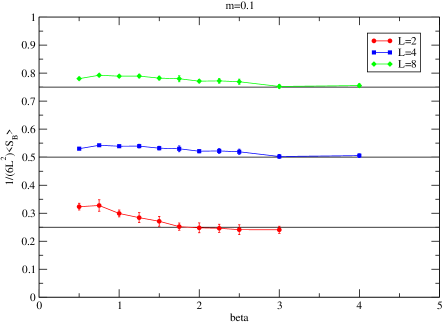
Figure 1: $\frac{\beta}{6L^{2}}<S_{B}>$

We have also examined the gauge action and the string tension determined by the smallest creutz ratio $\sigma=-\ln{W(1,1)W(2,2)/(W(1,2)W(2,1))}$ and plot these as a function of gauge coupling in the following plots ($m=0.1$ and $L=4$). These data are consistent with the existence of a confining phase.

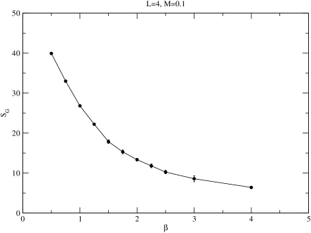
Figure 2: Gauge action for $U(2)$ model

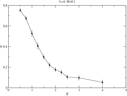
Figure 3: String tension for $U(2)$ model

7 Twisting ${\cal N}=4$ SYM in D=4

The ${\cal N}=4$ super Yang-Mills theory in four dimensions contains four Majorana spinors $\Psi^{I}_{\alpha}$ transforming under the Euclidean Lorentz group $SO(4)$ and an additional $SO_{R}(4)$ R-symmetry group. The Kähler-Dirac twist (see [31],[32]) consists of decomposing those fields into representations of the diagonal subgroup

$$SO(4)^{\prime}={\rm diag}(SO(4)\times SO(4)_{R})$$ (67)

As for two dimensions this twisting procedure is equivalent to regarding the supercharges and fermions as matrices:

$$\Psi = \eta I+\psi_{\mu}\gamma_{\mu}+\frac{1}{2!}\chi_{\mu\nu}\gamma_{\mu}\gamma_{\nu}+$$ (68)

$$+ \frac{1}{3!}\theta_{\mu\nu\lambda}\gamma_{\mu}\gamma_{\nu}\gamma_{\lambda}+\frac{1}{4!}\kappa_{\mu\nu\lambda\rho}\gamma_{\mu}\gamma_{\nu}\gamma_{\lambda}\gamma_{\rho}$$ (69)

To match the 16 real supercharges of the continuum theory it is natural to take these antisymmetric tensor fields real. They can then be regarded as the 16 grassmann components of a single real Kähler-Dirac field just as for two dimensions. There will now be a scalar nilpotent supercharge and corresponding bosonic superpartners $(\overline{\phi},A_{\mu},B_{\mu\nu},W_{\mu\nu\lambda},C_{\mu\nu\lambda\rho})$ In the end $B$ and $C$ will turn out to be multiplier fields and are integrated out of the final theory leaving two scalars $\overline{\phi}$, $\phi$ (which arises as a gauge parameter as in two dimensions), one vector $A_{m}u$ and the 4 independent components of $W_{\mu\nu\lambda}$. These latter four fields will combine with the two scalars to yield the usual 6 scalars of ${\cal N}=4$ super Yang-Mills.

The form of the $Q$-variations of these fields under the scalar supersymmetry can be obtained in analogy to the situation in two dimensions.

$$Q\overline{\phi} = \eta\;\;Q\eta=[\phi,\overline{\phi}]$$

$$QA_{\mu} = \psi_{\mu}\;\;Q\psi_{\mu}=-D_{\mu}\phi$$

$$QB_{\mu\nu} = [\phi,\chi_{\mu\nu}]\;\;Q\chi_{\mu\nu}=B_{\mu\nu}$$

$$QW_{\mu\nu\lambda} = \theta_{\mu\nu\lambda}\;\;Q\theta_{\mu\nu\lambda}=[\phi,W_{\mu\nu\lambda}]$$

$$QC_{\mu\nu\lambda\rho} = [\phi,\kappa_{\mu\nu\lambda\rho}]\;\;Q\kappa_{\mu\nu\lambda\rho}=C_{\mu\nu\lambda\rho}$$

$$Q\phi = 0$$ (70)

In deciding how to write down these transformations one is guided by the identification of physical fields. If a field is ultimately to be identified as a propagating field it is necessary to make its $Q$-variation yield another field. Multiplier fields vary into commutators. Notice again that the square of the supercharge is an infinitessimal gauge transformation parametrized by the field $\phi$.

We hypothesize that, following on from our general arguments, it should be possible to write the action as $Q$-exact function

$$S=\beta Q\Lambda$$ (71)

where the correct gauge fermion of ${\cal N}=4$ super Yang-Mills turns out to be

$$\Lambda = \int d^{4}x{\rm Tr}\left[\chi_{\mu\nu}\left(F_{\mu\nu}+\frac{1}{2}B_{\mu\nu}-\frac{1}{2}[W_{\mu\lambda\rho},W_{\nu\lambda\rho}]\right.\right.$$ (72)

$$+ \left.\left.D_{\lambda}W_{\lambda\mu\nu}\right)\right.$$

$$+ \left.\psi_{\mu}D_{\mu}\overline{\phi}+\frac{1}{4}\eta[\phi,\overline{\phi}]+\frac{1}{3!}\theta_{\mu\nu\lambda}[W_{\mu\nu\lambda},\overline{\phi}]\right.$$

$$+ \left.\frac{1}{4!}\kappa_{\mu\nu\lambda\rho}\left(\sqrt{2}D_{\left[\mu\right.}W_{\left.\nu\lambda\rho\right]}+\frac{1}{2}C_{\mu\nu\lambda\rho}\right)\right]$$

Several of these terms are in common with the gauge fermion of ${\cal N}=2$ super Yang-Mills theory in two dimensions. The new ones involve the $3$ and $4$-form fields. Of these the terms involving derivatives must be present to generate the correct Dirac-Kähler action for the twisted fermions (and will simultaneously generate the appropriate kinetic terms for the W-field). The commutator term involving $W_{\mu\nu\lambda}$ coupled to $\chi_{\mu\nu}$ will generate a quartic potential for the W-field analogous to that generated for the scalars $\phi$ and $\overline{\phi}$. This will allow contact to be made eventually with the supersymmetric theory where one expects the scalars and W-field to play similar roles. In the same way the commutator term involving $\overline{\phi}$ and $W$ will also generate the necessary mixed quartic couplings between the scalars and the W-field. Carrying out the $Q$-variation leads to the following action

$$S=\beta\left(S_{B}+S_{F}+S_{Y}\right)$$ (73)

where the piece of the action $S_{B}$ involving the bosonic fields takes the form

$$S_{B} = \int d^{4}x{\rm Tr}\left[B_{\mu\nu}\left(F_{\mu\nu}-\frac{1}{2}[W_{\mu\lambda\rho},W_{\nu\lambda\rho}]+D_{\lambda}W_{\lambda\mu\nu}+\frac{1}{2}B_{\mu\nu}\right)\right.$$ (74)

$$- \left.D_{\mu}\phi D_{\mu}\overline{\phi}+\frac{1}{4}[\phi,\overline{\phi}]^{2}-\frac{1}{3!}[\phi,W_{\mu\nu\lambda}][\overline{\phi},W_{\mu\nu\lambda}]\right.$$

$$+ \left.\frac{1}{4!}C_{\mu\nu\lambda\rho}\left(\sqrt{2}D_{\left[\mu\right.}W_{\left.\nu\lambda\rho\right]}+\frac{1}{2}C_{\mu\nu\lambda\rho}\right)\right]$$

and the fermion kinetic terms are given by $S_{F}$ with

$$S_{F} = \int d^{4}x{\rm Tr}\left[-\chi_{\mu\nu}D_{\left[\mu\right.}\psi_{\left.\nu\right]}-\chi_{\mu\nu}D_{\lambda}\theta_{\lambda\mu\nu}-\eta D_{\mu}\psi_{\mu}-\frac{\sqrt{2}}{4!}\kappa_{\mu\nu\lambda\rho}D_{\left[\mu\right.}\theta_{\left.\nu\lambda\rho\right]}\right]$$ (75)

and $S_{Y}$ contains the Yukawa couplings

$$S_{Y} = \int d^{4}x{\rm Tr}\left[-\frac{1}{4}\eta[\phi,\eta]-\frac{1}{2}\frac{1}{4!}\kappa_{\mu\nu\lambda\rho}[\phi,\kappa_{\mu\nu\lambda\rho}]-\frac{1}{2}\chi_{\mu\nu}[\phi,\chi_{\mu\nu}]\right.$$ (76)

$$+ \left.\psi_{\mu}[\overline{\phi},\psi_{\mu}]+\frac{1}{3!}\theta_{\mu\nu\lambda}[\overline{\phi},\theta_{\mu\nu\lambda}]\right.$$

$$+ \left.\frac{1}{3!}\eta[\theta_{\mu\nu\lambda},W_{\mu\nu\lambda}]-\frac{\sqrt{2}}{4!}\kappa_{\mu\nu\lambda\rho}[\psi_{\left[\mu\right.},W_{\left.\nu\lambda\rho\right]}]\right.$$

$$+ \left.\chi_{\mu\nu}[\theta_{\mu\lambda\rho},W_{\nu\lambda\rho}]-\chi_{\mu\nu}[\psi_{\lambda},W_{\lambda\mu\nu}]\right]$$

Integrating over the multiplier fields $B_{\mu\nu}$ and $C_{\mu\nu\lambda\rho}$ and subsequently utilizing the Bianchi identity leads to a new bosonic action of the form

$$S_{B} = \int d^{4}x{\rm Tr}\left[-\frac{1}{2}\left(\left(F_{\mu\nu}-\frac{1}{2}[W_{\mu\lambda\rho},W_{\nu\lambda\rho}]\right)^{2}+\left(D_{\lambda}W_{\lambda\mu\nu}\right)^{2}+\frac{2}{4!}\left(D_{\left[\mu\right.}W_{\left.\nu\lambda\rho\right]}\right)^{2}\right)\right.$$ (77)

$$- \left.D_{\mu}\phi D_{\mu}\overline{\phi}+\frac{1}{4}[\phi,\overline{\phi}]^{2}-\frac{1}{3!}[\phi,W_{\mu\nu\lambda}][\overline{\phi},W_{\mu\nu\lambda}]\right]$$

At this point it is useful to trade the $W$, $\theta$, and $\kappa$ fields for new variables which will allow contact to be made between this theory and one of the conventional twists of ${\cal N}=4$ super Yang-Mills. We write

$$W_{\mu\nu\lambda} = \epsilon_{\mu\nu\lambda\rho}V_{\rho}$$

$$\theta_{\mu\nu\lambda} = \epsilon_{\mu\nu\lambda\rho}\overline{\psi}_{\rho}$$

$$\kappa_{\mu\nu\lambda\rho} = \epsilon_{\mu\nu\lambda\rho}\overline{\eta}$$ (78)

In terms of these variables and after an additional integration by parts the bosonic action reads (notice that terms linear in $F_{\mu\nu}$ cancel)

$$S_{B} = \int d^{4}x{\rm Tr}\left[-\frac{1}{2}F^{2}_{\mu\nu}-\frac{1}{2}[V_{\mu},V_{\nu}]^{2}-\left(D_{\mu}V_{\nu}\right)^{2}\right.$$ (79)

$$- \left.D_{\mu}\phi D_{\mu}\overline{\phi}+\frac{1}{4}[\phi,\overline{\phi}]^{2}-[\phi,V_{\mu}][\overline{\phi},V_{\mu}]\right]$$

Making the additional rescalings $\chi\to 2\chi$ and $\overline{\eta}\to\frac{1}{\sqrt{2}}\overline{\eta}$ we find the fermion kinetic term takes the form

$$S_{F}=\int d^{4}x{\rm Tr}\left[-2\chi_{\mu\nu}D_{\left[\mu\right.}\psi_{\left.\nu\right]}-2\chi^{*}_{\mu\nu}D_{\left[\mu\right.}\overline{\psi}_{\left.\nu\right]}-2\frac{\eta}{2}D_{\mu}\psi_{\mu}-2\frac{\overline{\eta}}{2}D_{\mu}\overline{\psi}_{\mu}\right]$$ (80)

where $\chi^{*}_{\mu\nu}=\frac{1}{2}\epsilon_{\mu\nu\lambda\rho}\chi_{\lambda\rho}$ is the dual field. In these variables the Yukawa’s take on the more symmetrical form

$$S_{Y} = \int d^{4}x{\rm Tr}\left[-\frac{\eta}{2}[\phi,\frac{\eta}{2}]-\frac{\overline{\eta}}{2}[\phi,\frac{\overline{\eta}}{2}]-2\chi_{\mu\nu}[\phi,\chi_{\mu\nu}]\right.$$ (81)

$$+ \left.\psi_{\mu}[\overline{\phi},\psi_{\mu}]+\overline{\psi}_{\mu}[\overline{\phi},\overline{\psi}_{\mu}]\right.$$

$$+ \left.2\frac{\eta}{2}[\overline{\psi}_{\mu},V_{\mu}]-2\frac{\overline{\eta}}{2}[\psi_{\mu},V_{\mu}]\right.$$

$$+ 4\left.\chi_{\mu\nu}[\overline{\psi}_{\mu},V_{\nu}]-4\chi^{*}_{\mu\nu}[\psi_{\mu},V_{\nu}]\right]$$

The new action can be recognized as the twist of ${\cal N}=4$ super Yang-Mills due to Marcus [41].

Finally we will show how this twisted model may be reinterpreted in terms of the usual formulation of ${\cal N}=4$ super Yang-Mills theory. First, concentrate on the bosonic action and introduce the new fields ($\phi=\phi_{1}+i\phi_{2}$)

$$X^{\mu} = V_{\mu}\;\;\mu=0\ldots 3$$

$$X^{4} = \phi_{1}$$

$$X^{5} = \phi_{2}$$ (82)

Then the bosonic action may be trivially rewritten as

$$S_{B}=-\frac{1}{2}F^{2}_{\mu\nu}-\left(D_{\mu}X^{i}\right)^{2}-\frac{1}{2}\sum_{ij}[X_{i},X_{j}]^{2}$$ (83)

Notice this is real, positive semidefinite on account of the antihermitian basis for the fields. It is also precisely the bosonic sector of the ${\cal N}=4$ super Yang-Mills action with $X^{i}$ the usual $6$ real scalars of that theory [42].

Next let us turn our attention to the fermion kinetic term. From our previous discussion it should be clear that the twisted fermion kinetic term is nothing more than the component expansion of a Dirac-Kähler action:

$$S_{F}=\frac{1}{2}{\rm Tr}\Psi^{\dagger}\gamma.D\Psi$$ (84)

where $\Psi$ is the Dirac-Kähler field defined earlier with $\eta\to\eta/2$, $\theta_{\mu\nu\lambda}\to\epsilon_{\mu\nu\lambda\rho}\overline{\psi}_{\rho}$ and $\kappa_{\mu\nu\lambda\rho}\to\epsilon_{\mu\nu\lambda\rho}\overline{\eta}/2$. Naively such an action appears to describe a theory with four Dirac spinor fields - rather than the two one would have expected for ${\cal N}=4$ super Yang-Mills. However it is evident that $\Psi$ obeys a reality condition if its associated Dirac-Kähler field is real. This reduces the action to that of two degenerate Dirac fermions. To see this in detail let us adopt a Euclidean chiral basis for the $\gamma$-matrices

$$\begin{array}[]{cc}\gamma_{0}=\left(\begin{array}[]{cc}0&I\\ I&0\end{array}\right)&\gamma_{i}=\left(\begin{array}[]{cc}0&-i\sigma_{i}\\ i\sigma_{i}&0\end{array}\right)\end{array}$$ (85)

It is straightforward to see that the $\gamma$ matrices (and any products of them) obey a reality condition

$$\gamma_{\mu}^{*}=C\gamma_{\mu}C^{-1}$$ (86)

where the matrix $C$ is given by

$$C=\left(\begin{array}[]{cc}\sigma_{2}&0\\ 0&\sigma_{2}\end{array}\right)$$ (87)

With real p-form coefficients this implies a reality condition on $\Psi$ itself

$$\Psi^{*}=C\Psi C^{-1}$$ (88)

This in turn implies that $\Psi^{\dagger}=C\Psi^{T}C^{-1}$ which makes it clear that the result of integrating over the Dirac-Kähler field $\Psi$ should be the Pfaffian of the Dirac-Kähler operator (let us neglect the Yukawa couplings for the moment). This, in turn, will correspond to the product of two Dirac determinants.

To see this in more detail one can use the reality condition to show that successive columns $\Psi^{(n)}$ of $\Psi$ are not independent but are charge conjugates of each other

$$\Psi^{(2)}=C\left(\Psi^{(1)}\right)^{*}\;\;\Psi^{(4)}=C\left(\Psi^{(3)}\right)^{*}$$ (89)

These conditions allow us to rewrite the twisted fermion kinetic term in the conventional form

$$\frac{1}{2}\sum_{\alpha=1,2}\lambda^{\dagger}_{\alpha}\gamma.D\lambda_{\alpha}$$ (90)

where the spinors are read off as the first and third columns of the $\Psi$ matrix in this chiral basis:

$$\begin{array}[]{cc}\lambda_{1}=\left(\begin{array}[]{c}\frac{\eta}{2}-\frac{\overline{\eta}}{2}+2i\chi^{+}_{03}\\ -2\chi^{+}_{02}+2i\chi^{+}_{01}\\ \left(\psi_{0}+\overline{\psi}_{0}\right)+i\left(\psi_{3}+\overline{\psi}_{3}\right)\\ -\left(\psi_{2}+\overline{\psi}_{2}\right)+i\left(\psi_{1}+\overline{\psi}_{1}\right)\end{array}\right)&\lambda_{2}=\left(\begin{array}[]{c}\left(\psi_{0}-\overline{\psi}_{0}\right)+i\left(-\psi_{3}+\overline{\psi}_{3}\right)\\ \left(\psi_{2}-\overline{\psi}_{2}\right)+i\left(\overline{\psi}_{1}-\psi_{1}\right)\\ \frac{\eta}{2}+\frac{\overline{\eta}}{2}-2i\chi^{-}_{03}\\ 2\chi^{-}_{02}-2i\chi^{-}_{01}\end{array}\right)\\ \end{array}$$ (91)

Here, $\chi^{\pm}=\frac{1}{2}\left(\chi\pm\chi^{*}\right)$ are the usual self-dual and antiself-dual parts of the field. The Yukawa’s can also be put in the general form

$$\frac{1}{2}\sum_{\alpha=1,2}\lambda^{\dagger}_{\alpha}C^{\alpha}_{i}\Gamma^{i}[X^{i},\lambda_{\alpha}]$$ (92)

where $\Gamma^{i}=\left\{I,\gamma_{5},\gamma_{\mu}\gamma_{5},\mu=0\ldots 4\right\}$ and the coefficients $C^{\alpha}_{i}$ are just numbers. This is just the structure expected of ${\cal N}=4$ super Yang-Mills. Notice that both Dirac operators $M^{\alpha}$ including the Yukawa interactions possess the symmetry

$$\left(D^{\alpha}\right)^{*}=CD^{\alpha}C^{-1}$$ (93)

which shows that their eigenvalues come in complex conjugate pairs and hence the associated determinants are positive definite.

8 Lattice ${\cal N}=4$ super Yang-Mills

The lattice action is obtained by discretization of the $Q$-exact action given in eqn. 72. Notice it is important not to use the same dual variables as Marcus in discretizing the theory as the duality transformation is not compatible with the lattice gauge transformations we have described. With that proviso the prescription is essentially the same as for the two dimensional theory [31]. We list it now for a $D$-dimensional theory.

• A continuum p-form field $f_{\mu_{1}\ldots\mu_{p}}(x)$ will be mapped to a corresponding lattice field associated with the $p$-dimensional hypercube at lattice site $x$ spanned by the (positively directed) unit vectors $\{\mu_{1}\ldots\mu_{p}\}$.

• Such a lattice field is taken to transform under gauge transformations in the following way

  $$f_{\mu_{1}\ldots\mu_{p}}(x)\to G(x)f_{\mu_{1}\ldots\mu_{p}}(x)G^{-1}(x+e_{\mu_{1}\ldots\mu_{p}})$$ (94)

  where the vector $e_{\mu_{1}\ldots\mu_{p}}=\sum_{j=1}^{p}\mu_{j}$.

• To construct gauge invariant quantities we will need to introduce both $f_{\mu_{1}\ldots\mu_{p}}$ and its hermitian conjugate $f^{\dagger}_{\mu_{1}\ldots\mu_{p}}(x)$. The latter transforms as

  $$f^{\dagger}_{\mu_{1}\ldots\mu_{p}}(x)\to G(x+e_{\mu_{1}\ldots\mu_{p}})f_{\mu_{1}\ldots\mu_{p}}(x)G^{-1}(x)$$ (95)

  Since for all fields bar the gauge field we will assume $f_{\mu_{1}\ldots\mu_{p}}=\sum_{a}f^{a}_{\mu_{1}\ldots\mu_{p}}T^{a}$ where $T^{a}$ are antihermitian generators of $U(N)$, this necessitates taking the fields $f^{a}_{\mu_{1}\ldots\mu_{p}}$ to be complex.

• For a continuum gauge field we introduce lattice link fields $U_{\mu}(x)=e^{A_{\mu}(x)}=e^{A^{a}_{\mu}(x)T^{a}}$ with $A^{a}_{\mu}(x)$ complex together with its conjugate $U^{\dagger}_{\mu}=e^{A^{\dagger}_{\mu}(x)}$.

• A covariant forward difference operator can be defined which acts on a field $f_{\mu_{1}\ldots\mu_{p}}(x)$ as follows

  $$D^{+}_{\mu}f_{\mu_{1}\ldots\mu_{p}}(x)=U_{\mu}(x)f_{\mu_{1}\ldots\mu_{p}}(x+\mu)-f_{\mu_{1}\ldots\mu_{p}}(x)U_{\mu}(x+e_{\mu_{1}\ldots\mu_{p}})$$ (96)

  This operator acts like a lattice exterior derivative with respect to gauge transformations in mapping a $p$-form lattice field to a $(p+1)$-form lattice field.

• Similarly we can define an adjoint operator $D^{-}_{\mu}$ whose action on some field $f_{\mu_{1}\ldots\mu_{p}}$ is given by

  $$D^{-}_{\mu}f_{\mu_{1}\ldots\mu_{p}}(x)=f_{\mu_{1}\ldots\mu_{p}}(x)U^{\dagger}_{\mu}(x+e_{\mu_{1}\ldots\mu_{p}}-\mu)-U^{\dagger}_{\mu}(x-\mu)f_{\mu_{1}\ldots\mu_{p}}(x-\mu)$$ (97)

  It thus acts like the adjoint of the exterior derivative.

• As for two dimensions all instances of $\partial_{\mu}$ in the continuum action will be replaced by $D^{+}_{\mu}$ if the derivative acts like $d$ (curl-like operation) and $D^{-}_{\mu}$ if the derivative acts like $d^{\dagger}$ (divergence-like operation).

This prescription preserves the twisted scalar supersymmetry and gauge invariance and targets a complexified version of the ${\cal N}=4$ super Yang-Mills model. Again, to obtain ${\cal N}=4$ SYM we conjecture that the Ward identities corresponding to the scalar supersymmetry will be satisfied without fine tuning in the continuum limit $\beta\to\infty$ for the truncated lattice model in which the fields are taken real.

9 Conclusions

In this paper we have presented a new way to put supersymmetric theories on the lattice. The approach only works for theories with a number of supercharges which is a integer multiple of $2^{D}$ if $D$ is the dimension of (Euclidean) spacetime. This includes the important cases of ${\cal N}=2$ and ${\cal N}=4$ super Yang-Mills theory in two and four dimensions respectively. The basic idea is to start from a twisted formulation of the supersymmetric theory in which the fermions are represented as grassmann valued antisymmetric tensor fields. The original supersymmetry algebra is replaced by a twisted algebra which contains a scalar nilpotent supercharge $Q$. Furthermore the action of the theory can then be written as the $Q$-variation of some function. It is straightforward to generalize the action of the scalar supersymmetry to the lattice while maintaining its nilpotent property. Invariance of the lattice theory under the scalar supersymmetry can then be obtained easily. We have described the details of our discretization prescription in detail. It requires the introduction of particular covariant forward and backward difference operators and non standard gauge transformation properties of the fields. The final theory is gauge invariant, free of spectrum doubling and possesses an exact supersymmetry. The price one pays for this is that the lattice fields are in general complexified. We have argued that the $Q$-exactness of the action ensures nevertheless that the theory truncated to the real line will satisfy the Ward identities corresponding to the scalar supersymmetry without fine tuning in the continuum limit. We have also presented preliminary numerical results stemming from a dynamical fermion simulation of the $D=2$ $U(2)$ model using the new RHMC algorithm.

There are several directions for further work. The most obvious is the need for both perturbative and numerical checks of both the exact and broken Ward identities corresponding to the twisted supersymmetry. Exactly how much residual fine tuning would be required in the four dimensional theory is currently unclear and could be revealed by such an analysis. It should also be possible to use these ideas to construct lattice regularizations for the ${\cal N}=4,8$ theories in two dimensions and the ${\cal N}=8$ theory in three dimensions. This would allow contact to be made with predictions from string theory and supergravity theories in lattice models which could be simulated relatively easily and with high precision. The geometrical nature of the twisted theory lends one to speculate that it should be possible to formulate these models on general simplicial lattices. If this could be realized, then the resulting models could be coupled to gravity in the usual way by carrying out a sum over random lattices resulting in a lattice regulated supergravity theory. It would also be very interesting to understand the relationship, if any, between twisting and the orbifold constructions of Kaplan at al.

It appears that the twisted formulation of a theory with extended supersymmetry affords a more useful starting point for constructing lattice models over conventional approaches based on spinors. However, the precise details of the discretization procedure are not determined uniquely. While this work was in preparation a new paper by D’Adda et al [43] was posted which claims to maintain all the supercharges of the two dimensional twisted theory by adopting a different mapping of the continuum twisted theory to the lattice. This appears to be a very intriguing development.

References

- [1] The Quantum Theory of Fields Vol. III Supersymmetry, S. Weinberg, Cambridge University Press (2000).
- [2] N. Seiberg and E. Witten, Nucl. Phys. B431 (1994) 484.
- [3] E. Martinec and V. Sahakian, hep-th/9810224, L. Susskind, hep-th/9805115, O. Aharony, J. Marsano, S. Minwalla and T. Wiseman, hep-th/0406210, N. Itzhaki, J. Maldacena, J. Sonnenschein and S. Yankielowicz, hep-th/9802042.
- [4] J.M. Maldecena, Adv. Theor. Math. Phys. 2 (1998) 231 [Int. J. Theor. Phys 38 (1999) 1113].
-
[5]
P. Dondi and H. Nicolai, Nuovo Cimento 41A (1977)
S. Elitzur and A. Schwimmer, Nucl. Phys. B226 (1983) 109 J. Bartels and J. Bronzan, Phys. Rev. D28 (1983) 818.
T. Banks and P. Windey, Nucl. Phys. B198 (1982) 226.
I. Montvay, Nucl. Phys. B466 (1996) 259.
M Golterman and D. Petcher, Nucl. Phys. B319 (1989) 307.
W. Bietenholz, Mod. Phys. Lett A14 (1999) 51. H. Aratyn and A.H. Zimerman, J. Phys. A 18 (1985) L487. (1985) 225
Y. Kikukawa and Y. Nakayama, Phys. Rev. D66 (2002) 094508.
K. Fujikawa, Phys. Rev. D66 (2002) 074510.
J. Nishimura, Phys. Lett. B406 (1997) 215.
S. Catterall and S. Karamov, Phys. Rev. D 68 (2003) 014503.
W. Bietenholtz, Mod. Phys. Lett. A14 (1999) 51.
M. Beccaria, M. Campostrini, G.De Angelis and A. Feo, Phys. Rev. D70 (2004)
M. Beccaria, M. Campostrini, A. Feo, Phys. Rev. D69 (2004) 095010.
H. Aratyn, M. Goto and A.H. Zimerman, Nuovo Cimento A88 -
[6]
A. Feo, Supersymmetry on the Lattice, hep-lat/0210015
- [7] D. B. Kaplan, Recent Developments in Lattice Supersymmetry, hep-lat/0309099
- [8] M. Bonini and A. Feo, JHEP 0409 (2004) 011.
- [9] super Yang-Mills on a (3+1) dimensional transverse lattice, M. Harada, S. Pinsky, hep-lat/0411024, M. Harada, S. Pinsky, Phys. Rev. D70 (2004) 087701, M. Harada, S. Pinsky, Phys. Lett. B567 (2003) 277
- [10] D.B. Kaplan, E. Katz and M. Unsal, JHEP 0305 (2003) 037, A.G. Cohen, D.B. Kaplan, E. Katz, M. Unsal, JHEP 0308 (2003) 024, A.G. Cohen, D.B. Kaplan, E. Katz, M. Unsal, JHEP 0312 (2003) 031
- [11] D. B. Kaplan and M. Unsal, hep-lat/0503039.
- [12] M. Unsal, hep-lat/0504016.
-
[13]
J. Nishimura, S. Rey and F. Sugino, JHEP 0302 (2003) 032
J. Giedt, E. Poppitz and M. Rozali, JHEP 0303 (2003) 035
J. Giedt, Nucl. Phys. B668 (2003) 138
J. Giedt, Nucl. Phys. B674 (2003) 259. - [14] S. Catterall, JHEP 0305 (2003) 038.
- [15] J. Giedt, E. Poppitz, hep-lat/0407135.
- [16] A. D’Adda, I. Kamamori, N. Kawamoto, K. Nagata, hep-lat/0406029.
- [17] S. Catterall and E. Gregory, Phys. Lett. B487 (2000) 349.
- [18] Giedt, Koniuk, Poppitz and Yavin, JHEP 0412 (2004) 033.
- [19] S. Catterall and S. Karamov, Phys. Rev. D65 (2002) 094501.
- [20] Giedt, hep-lat/0507016.
- [21] S. Catterall and S. Ghadab, JHEP 0405 (2004) 044.
- [22] F. Sugino, JHEP 0401 (2004) 015.
- [23] F. Sugino, JHEP 0403 (2004) 067.
- [24] E. Witten, Comm. Math. Phys. 117 (1988) 353.
- [25] N. Kawamoto , T. Tsukioka, Phys. Rev. D61 (105009) 2000.
- [26] J. Kato, N. Kawamoto and Y. Uchida, Int. J. Mod. Phys. A19 (2004) 2149.
- [27] S. Catterall, Nucl. Phys. B Proceedings Suppl. 140 (2005) 751
- [28] S. Catterall, JHEP 0411 (2004) 006.
- [29] D. Birmingham, M. Blau, M. Rakowski and G. Thompson, Phys. Rep. 209, numbers 4 and 5 (1991) 129.=
- [30] T. Banks, Y. Dothan and D. Horn, Phys. Lett. B117 (1982) 413.
- [31] S. Catterall, JHEP 06 027 (2005).
- [32] D’Adda, Kanamori, Kawamoto and Nagata, Nucl. Phys. B707 (2005) 100.
- [33] S. Elitzur, E. Rabinovici and A. Schwimmer, Phys. Lett B119 (1982) 165.
- [34] H. Aratyn, M. Goto and A.H. Zimerman, Nuovo Cimento A84, (1984) 255
-
[35]
P. Becher, Phys. Lett. B104 (1981) 221
P. Becher and H. Joos, Z. Phys. C 15 (1982) 343. - [36] J. Rabin, Nucl. Phys. B201 (1982) 315.
- [37] M. Clark and A. Kennedy, hep-lat/0409133.
- [38] S. Duane, A. Kennedy, B. Pendleton and D. Roweth, Phys. Lett. B195B (1987) 216.
- [39] B. Jegerlehner, Krylov solvers for shifted linear systems hep-lat/9612014
- [40] Numerical study of twisted super Yang-Mills, S. Catterall, in preparation.
- [41] N. Marcus, Nucl. Phys. B452 (1995) 331.
- [42] E. D’Hoker and D. Freedman, hep-th/0201253.
- [43] D’Adda, Kanamori, Kawamoto and Nagata, hep-lat/0507029.