Heavy quark masses from Fermilab Fermions

Abstract:

Using automated perturbation theory techniques, we have computed the one-loop mass of Fermilab fermions, with an improved gluon action. We will present the results of these calculations, and the resulting predictions for the charm and bottom quark masses in the MSbar scheme. We report $\overline{m}_{c}(\overline{m}_{c})=1.22(9)$ GeV and $\overline{m}_{b}(\overline{m}_{b})=4.7(4)$ GeV. In addition we present results for the one-loop coefficients of the Fermilab action.

PoS(LAT2005)209

In recent years there has been a lot of progress in lattice perturbation theory [1, 2]. In particular, the implementation of automated perturbation theory routines has allowed many problems to be tackled. Lattice perturbation theory has many applications, for example the determinations of improvement coefficients and renormalization factors. In addition, lattice perturbation theory is used in connecting non-perturbative simulations to quantities of interest to the wider high-energy community. An example of this is the recent determination of the strong coupling constant $\alpha_{s}$ [3].

In this report we present results of our one-loop calculations of current renormalizations, action parameters and quark masses for the Fermilab fermion action [4]. The lattice perturbation theory produces an estimate of the quark’s pole mass. This can be converted into the $\overline{MS}$ scheme at some scale $\mu$. We give a few details of this conversion and report preliminary values for the quark masses. These are compared to the PDG values.

Simulating heavy quarks on the lattice poses a special problem because the scale $m_{0}a$ is not small for typical lattice spacings. For actions designed for light quarks $\mathcal{O}(m_{0}a)$ errors can be large. There are a few different approaches to this problem. One popular one is the Fermilab approach, which resums all mass dependance into the coefficients in the action.

The Fermilab action is

$$S = a^{4}\sum_{x}\bar{\psi}(x)\left[m_{0}+\frac{1+\gamma_{4}}{2}D_{4}^{-}-\frac{1-\gamma_{4}}{2}D_{4}^{+}+\zeta\vec{\gamma}\cdot\vec{D}\right.$$ (1)

$$- \left.\frac{ar_{s}\zeta}{2}\triangle^{(3)}-\frac{iac_{B}\zeta}{2}\vec{\Sigma}\cdot\vec{B}-\frac{ac_{E}\zeta}{2}\vec{\alpha}\cdot\vec{E}\right]\psi(x)$$

where definitions of the various operators can be found in [4]. This action is designed to smoothly interpolate between the zero mass and infinite-mass limits. As such it is ideal for simulations of charm quarks, where other methods (such as NRQCD) might have problems [5]. All the coefficients in the Fermilab action are mass dependent, however at tree level we can use

$$\zeta=r_{s}=c_{E}=c_{B}=1.$$ (2)

Using our automated perturbation theory techniques we have completed all the “basic” one-loop calculations for this action. These are the mass and wavefunction renormalizations, the renormalization of heavy-light and heavy-heavy vector and axial vector currents and the one-loop matching of the action parameters $c_{B}$ and $c_{E}$. In the following sections we will present results for the action parameters and the mass renormalizations.

All of the calculations presented here were carried out with using our automated perturbation theory codes. Apart from the wavefunction renormalization all these quantities are infrared finite and gauge invariant. Infrared divergences in individual diagrams were regulated by using a gluon mass.

To match the coefficients $c_{B}(c_{E})$ we compute the scattering of a quark off of a background chromo-magentic(electric) field in both the lattice and continuum field theories, then tune the action parameters until the difference vanishes. The relevant diagrams are shown in figure 1.

One interesting feature of our calculation is the use of lattice to lattice matching [6]. Rather than computing the continuum contribution using standard methods, we use a simple lattice theory, with a spacing $a^{\prime}$ that is driven very small. Figure 2 illustrates this for two cases, naive fermions (which have a quadratic approach to $a^{\prime}=0$) and Wilson fermions (which have a linear $a\to 0$ behaviour). What is shown in figure 2 is actually the difference between the two sets of diagrams (Fermilab at spacing $a$ and Wilson/naive at spacing $a^{\prime}$) there are additional counterterms in the matching coming from the one loop part of $\zeta$, [7] has details. One sees that the same result for the matching coefficient $\delta_{B}$ is obtained using the continuum limit ($a^{\prime}\to 0$) of either Wilson or naive quarks for the continuum side of the matching.

The one-loop contribution to $c_{B}$ is plotted in figure 3. The results for $c_{E}$ are very similar. It is clear from the figure that the result, when tadpole improved, is nearly zero over the whole range of interesting masses ($0<m_{0}a<2$). This means that errors due to using only the tree level action parameters have likely been overestimated. This conclusion only applies if the action has been tadpole improved. The unimproved coefficients are quite large.

To date all lattice determinations of the hyperfine splittings in the $J/\phi$ system have come out too low ([8] and [9]). These splittings are quite sensitive to the coefficient of $\Sigma\cdot B$ so it was believed that the one-loop determination of $c_{B}$ would bring the splittings up. This is not the case, the one-loop coefficient is very small. However, there is evidence [9] that the discrepancy in the hyperfine splittings is decreasing as $a\to 0$. A determination with the fully $\mathcal{O}(a^{2})$ improved Fermilab action [10] would be very useful.

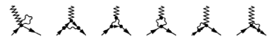
Figure 1: Diagrams for matching action parameters

Figure 2: One loop lattice to lattice matching of $\delta_{B}=c_{B}-\rm{counterterms}$ at $m_{0}a=0.1$, with improved glue.

Figure 3: The one-loop coefficient of $\Sigma\cdot B$, with and without tadpole improvement

In addition to the action parameters, we have computed the quark masses for the Fermilab action. This calculation is similar to [11], however we have used the Symanzik improved gluon action. There are two masses to compute in the Fermilab formalism, the rest mass $M_{1}$ and the kinetic mass $M_{2}$. These are defined via the small $pa$ expansion of the quark energy

$$E=M_{1}+\frac{\bf{p}^{2}}{2M_{2}}+\mathcal{O}(p^{4}a^{4}).$$ (3)

The rest mass has the perturbative expansion $M_{1}=M_{1}^{[0]}+\alpha_{V}(q^{*})M_{1}^{[1]}+\cdots$ where $M_{1}^{[0]}=\log(1+m_{0}a)$ and $\alpha_{V}(q^{*})$ is the QCD coupling in the V scheme evaluated at the BLM [12] scale. The kinetic mass is usually expressed as follows

$$M_{2}=Z_{M_{2}}\frac{\exp{M_{1}}\sinh M_{1}}{1+\sinh M_{1}}$$ (4)

where $M_{1}$ is the all orders rest mass and

$$Z_{M_{2}}=1+\alpha_{V}(q^{*})Z_{M_{2}}^{[1]}+\cdots.$$ (5)

Figures 4 and 5 show the one loop coefficients of the rest mass and the kinetic mass factor $Z_{M_{2}}$ over a wide range of input bare masses. In all cases the we see a smooth transition from the small to large mass limits.

Figure 4: The one-loop rest mass, with and without tadpole improvement

Figure 5: The one-loop kinetic mass renormalization

The values $M_{1}$ and $M_{2}$ can be used to provide two different estimates of the pole mass of the quark [13]. The first method is to estimate the binding energy, $B_{1}a=M_{1}^{\bar{Q}Q^{\prime},\rm{latt}}-N_{Q}M_{1}a$, where $M_{1}^{\bar{Q}Q^{\prime},\rm{latt}}$ is a spin average meson mass computed on the lattice ($J/\psi/\eta_{c}$ for the $c$ quark, $B_{s}/B_{s}^{*}$ for the $b$ quark) and $N_{Q}$ is the number of heavy quarks in the meson (2 and 1, respectively). The pole mass is then $m_{\rm{pole}}=M^{\bar{Q}Q^{\prime},\rm{expt}}-B_{1}$, where $M^{\bar{Q}Q^{\prime},\rm{expt}}$ is the meson mass taken from experiment. Beyond the truncation of the perturbation series this method suffers from two major sources of error. The first is that one needs to divide out the lattice spacing $a$, and the second is that it is quite sensitive to the bare mass $m_{0}$ used as input.

The second method for estimating the pole mass does not suffer from these errors. One begins with a perturbative determination of $M_{2}a$ and takes

$$m_{\rm{pole}}=\left(M_{2}a\right)^{\rm{PT}}\frac{M^{\bar{Q}Q^{\prime},\rm{expt}}}{M^{\bar{Q}Q^{\prime},\rm{latt}}a}.$$ (6)

This method avoids the errors of the method one, the dependance on the lattice spacing cancels and a small mistuning of the bare mass largely cancels in the ratio.

Once we have a value for the pole mass we can convert it into a value for the $\overline{MS}$ mass at some scale $\mu$ using

$$m_{\rm{pole}}=\overline{m}(\mu)\left\{1+\frac{4}{3\pi}\left[1+\log\left(\frac{\mu^{2}}{m_{0}^{2}}\right)\right]\alpha_{V}(q^{*})\right\}$$ (7)

We follow the conventional practice, and quote $\overline{m}(\mu)$ at the scale of the $\overline{MS}$ mass itself, $\mu=\overline{m}$. We use the BLM method to determine the scale $q^{*}$ in the coupling $\alpha_{V}(q^{*})$. We estimate the relative systematic error coming from the neglected higher-orders in the perturbative matching as $\pm\alpha_{V}^{2}(q^{*})$. We obtain

$$\overline{m}^{\rm{method1}}_{c}(\overline{m}_{c}) = 1.24(1)(9)\,\rm{GeV}\quad\rm{Fine}$$ (8)

$$\overline{m}^{\rm{method2}}_{c}(\overline{m}_{c}) = 1.22(0)(9)\,\rm{GeV}\quad\rm{Fine}$$ (9)

$$\overline{m}^{\rm{method1}}_{c}(\overline{m}_{c}) = 1.39(1)(13)\,\rm{GeV}\quad\rm{Coarse}$$ (10)

$$\overline{m}^{\rm{method2}}_{c}(\overline{m}_{c}) = 1.30(0)(12)\,\rm{GeV}\quad\rm{Coarse}$$ (11)

$$\overline{m}^{\rm{method1}}_{b}(\overline{m}_{b}) = 4.4(1)(3)\,\rm{GeV}\quad\rm{Fine}$$ (12)

$$\overline{m}^{\rm{method2}}_{b}(\overline{m}_{b}) = 4.7(0)(4)\,\rm{GeV}\quad\rm{Fine}$$ (13)

where the first error is from the determination of the lattice spacing (which only affects method one) and the second our estimate of the unknown two-loop error.

Our best values are the method two determinations on the fine lattice, which compare well with the PDG values $\overline{m}^{\rm{PDG}}_{c}(\overline{m}_{c})=1.25(10)$ GeV and $\overline{m}^{\rm{PDG}}_{b}(\overline{m}_{b})=4.25(15)$ GeV. These results are based on preliminary values for the input masses [14] so they may change somewhat.

In this report we have presented results for the action parameters and masses of Fermilab fermions to one-loop. For truly high precision determinations two-loop precision will be needed. These calculations are in progress.

References

- [1] H. D. Trottier, Higher-order perturbation theory for highly-improved actions, Nucl. Phys. Proc. Suppl. 129 (2004) 142–148 [hep-lat/0310044].
- [2] Q. Mason, High precision fundamental constants using lattice perturbation theory, . PoS(LAT2005)011.
- [3] HPQCD Collaboration, Q. Mason et. al., Accurate determinations of alpha(s) from realistic lattice qcd, Phys. Rev. Lett. 95 (2005) 052002 [hep-lat/0503005].
- [4] A. X. El-Khadra, A. S. Kronfeld and P. B. Mackenzie, Massive fermions in lattice gauge theory, Phys. Rev. D55 (1997) 3933–3957 [hep-lat/9604004].
- [5] H. D. Trottier, Quarkonium spin structure in lattice nrqcd, Phys. Rev. D55 (1997) 6844–6851 [hep-lat/9611026].
- [6] M. A. Nobes and H. D. Trottier, Progress in automated perturbation theory for heavy quark physics, Nucl. Phys. Proc. Suppl. 129 (2004) 355–357 [hep-lat/0309086].
- [7] M. A. Nobes, Automated Perturbation Theory for Improved Quark and Gluon Actions. PhD thesis, Simon Fraser University, 2004.
- [8] C. Stewart and R. Koniuk, Unquenched charmonium with nrqcd, Phys. Rev. D63 (2001) 054503 [hep-lat/0005024].
- [9] S. Gottlieb, Onium masses with three flavors of dynamical quarks, . PoS(LAT2005)203.
- [10] M. B. Oktay, A. X. El-Khadra, A. S. Kronfeld and P. B. Mackenzie, A more improved lattice action for heavy quarks, Nucl. Phys. Proc. Suppl. 129 (2004) 349–351 [hep-lat/0310016].
- [11] B. P. G. Mertens, A. S. Kronfeld and A. X. El-Khadra, The self energy of massive lattice fermions, Phys. Rev. D58 (1998) 034505 [hep-lat/9712024].
- [12] K. Hornbostel, G. P. Lepage and C. Morningstar, Scale setting for beyond leading order, Phys. Rev. D67 (2003) 034023 [hep-ph/0208224].
- [13] A. S. Kronfeld, The charm quark’s mass, Nucl. Phys. Proc. Suppl. 63 (1998) 311–313 [hep-lat/9710007].
- [14] J. Simone, M. Okamoto and S. Gottlieb, “Heavy quark mass tuning.” Private communication.