Chiral limit of 2-color QCD at strong couplings

Abstract:

We study two-color lattice QCD with massless staggered fermions in the strong coupling limit using a new and efficient cluster algorithm. We focus on the phase diagram of the model as a function of temperature $T$ and baryon chemical potential $\mu$ by working on $L_{t}\times L^{d}$ lattices in both $d=2,3$. In $d=3$ we find that at $\mu=0$ the ground state of the system breaks the global $U(2)$ symmetry present in the model to $U(1)$, while the finite temperature phase transition (with $L_{t}=4$) which restores the symmetry is a weak first order transition. In $d=2$ we find evidence for a novel phase transition similar to the Berezinky-Kosterlitz-Thouless phenomena. On the other hand the quantum ($T=0$) phase transition to a symmetric phase as a function of $\mu$ is second order in both $d=2,3$ and belongs to the mean field universality class.

PoS(LAT2005)147

1 INTRODUCTION

Two-color QCD has been extensively studied over the years both theoretically [1, 2, 3, 4] and numerically [5, 6, 7, 8, 9, 10, 11, 12]. Although a lot of progress has been made in uncovering important qualitative features of this theory, many interesting quantitative questions remain:

1. What is the order of the finite temperature chiral transition at zero and non-zero chemical potentials?

2. Can the low energy physics at small $T$ and $\mu$ be captured by chiral perturbation theory? An answer to this question was attempted in [11].

3. What is the order of the phase transition that occurs when the lattice gets saturated with baryons at $T=0$?

4. What is the phase structure in two spatial dimensions since spontaneous symmetry breaking is forbidden at finite temperatures.

The reason for the lack of quantitative progress can be traced to the fact that all previous studies have been limited to small lattice sizes and relatively large quark masses; a problem which haunts all numerical studies of strongly correlated fermionic systems.

In this work we try to make progress by considering the strong coupling limit. Although this limit has the worst lattice artifacts, it contains some of the essential physics, namely confinement and chiral symmetry breaking. On the other hand recent advances in Monte Carlo algorithms allow us to study the chiral limit on large lattices with relative ease in the strong coupling limit [13]. In this work we extend these algorithms and apply it to study strong coupling two-color QCD with staggered fermions. This theory is especially interesting due to an enhanced $U(2)$ symmetry at zero quark mass and baryon chemical potential. It was originally considered in [14, 15] and was recently reviewed in [16]. However, many of the questions raised above remain unanswered even in this simplified limit.

2 THE MODEL

Our model lives on a $d+1$ dimensional hyper-cubic lattice with sites $x\equiv(x_{t};x_{1},x_{2},..,x_{d})$. The size of the lattice is taken to be $L_{t}\times L^{d}$ and is periodic in all directions. The action of our model is

$$S=-\sum_{x,\alpha}r_{\alpha}\eta_{\alpha}(x)\Bigg{[}e^{\mu a_{t}\delta_{t,\alpha}}\overline{\chi}(x)U_{\alpha}(x)\chi(x+\hat{\alpha})-e^{-\mu a_{t}\delta_{t,\alpha}}\overline{\chi}(x+\hat{\alpha})U_{\alpha}^{\dagger}(x)\chi(x)\Bigg{]}.$$ (1)

The Grassmann fields $\overline{\chi}(x)$ and $\chi(x)$ represent row and column vectors with $2$ color components associated to the lattice site $x$. The color component of the quark fields will be denoted as $\chi_{a},a=1,2$. The gauge fields $U_{\alpha}(x)$ are elements of $SU(2)$ group and live on the links between $x$ and $x+\hat{\alpha}$ where $\alpha=1,2,..,d$ for spatial links and $\alpha=t$ for temporal link. The factor $r_{\alpha}=1$ for $\alpha=1,2,..,d$ and $r_{t}=\frac{1}{a_{t}}$ with $a_{t}$ being the asymmetry factor between spatial and temporal lattice spacing. This asymmetry allows us to study finite temperature behavior [17].

A discussion of the relevant symmetries of the action (1) can be found in [8, 16]. As explained in these references when $\mu=0$ our model has a $U(2)$ global symmetry:

$$X_{o}\rightarrow VX_{o},\quad\overline{X}_{e}\rightarrow\overline{X}_{e}V^{\dagger},\qquad V=\exp(i\vec{\alpha}\cdot\vec{\sigma}+i\phi)\in U(2).$$ (2)

where $\overline{X}_{e}$ and $X_{o}$ are given by

$$\overline{X}_{e}=(\overline{\chi}_{e},-\chi_{e}^{tr}\tau_{2}),\quad\quad X_{o}=\left(\begin{array}[]{c}\chi_{o}\cr-\tau_{2}\overline{\chi}_{o}^{tr}\end{array}\right)$$ (3)

and the subscripts $e$ and $o$ refer to even and odd sites. Note in our notation $\vec{\sigma}$ are Pauli matrices that mix $\chi$ and $\overline{\chi}^{tr}$ present in $X_{o}$ and $\overline{X}_{e}$ while $\vec{\tau}$ are Pauli matrices that act on the color space. The $U(2)$ symmetry is reduced to $U_{B}(1)\times U_{\chi}(1)$ in the presence of a chemical potential:

$$\begin{array}[]{ll}U_{B}(1):&\quad\quad X_{o}\rightarrow\exp(i\sigma_{3}\phi)X_{o},\quad\overline{X}_{e}\rightarrow\overline{X}_{e}\exp(-i\sigma_{3}\phi)\cr U_{\chi}(1):&\quad\quad X_{o}\rightarrow\exp(i\phi)X_{o},\quad\overline{X}_{e}\rightarrow\overline{X}_{e}\exp(-i\phi).\end{array}$$ (4)

Here $U_{B}(1)$ is the baryon number symmetry $\chi(x)\rightarrow\mathrm{e}^{i\phi}\chi(x),\quad\overline{\chi}(x)\rightarrow\overline{\chi}(x)\mathrm{e}^{-i\phi}$ and $U_{\chi}(1)$ is the chiral symmetry of staggered fermions $\chi(x)\rightarrow\mathrm{e}^{i\phi\varepsilon(x)}\chi(x)$, $\overline{\chi}(x)\rightarrow\overline{\chi}(x)\mathrm{e}^{i\phi\varepsilon(x)}$ where $\varepsilon(x)=(-1)^{x_{t}+x_{1}+x_{2}+...+x_{d}}$.

3 DIMER-BARYONLOOP REPRESENTATION

One of the computational advantages of the strong coupling limit is that in this limit it is possible to rewrite the partition function,

$$Z=\int[DU][d\overline{\chi}d\chi]\exp(-S),$$ (5)

as a sum over configurations containing gauge invariant objects [18, 19, 20]. In our case these objects turn out to be dimers and baryonloops. A lattice configuration $K$ of dimers and baryonloops is constructed as follows:

• Every link of the lattice connecting the site $x$ with the neighboring site $x+\hat{\alpha}$ contains either a dimer $k_{\alpha}(x)=0,1,2$ or a directed baryonic bond $b_{\alpha}(x)=-1,0,1$. $b_{\alpha}(x)=1$ indicates the direction is from $x$ to $x+\hat{\alpha}$ and $-1$ implies it is from $x+\hat{\alpha}$ to $x$. $k_{\alpha}(x)=0$ and $b_{\alpha}(x)=0$ means that the link does not contain any dimer or baryonic bond. In our notation we also allow $\hat{\alpha}$ to be negative. Thus, if $\alpha$ was positive, $k_{-\alpha}(x)$ and $b_{-\alpha}(x)$ will represent dimers and baryonic bonds connecting $x$ with $x-\hat{\alpha}$.

• If a site is connected to a baryonic bond then it must have exactly one incoming baryonic bond and one outgoing baryonic bond. Thus baryonic bonds always form self-avoiding baryonloops.

• Every lattice site $x$ that does not contain a baryonic bond must satisfy the constraint

  $$\sum_{\alpha}k_{\alpha}(x)=2$$

  where the sum includes negative values of $\alpha$.

An example of a dimer-baryonloop configuration is shown in Figure 1.

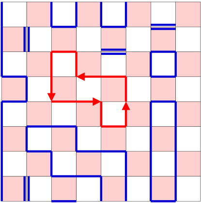
Figure 1: An example of a dimer-baryonloop configuration.

Note that sites connected by $k_{\alpha}(x)=1$ also form loops. Given the set $\{K\}$ of such dimer-baryonloop configurations the partition function of the theory described by eq.(1) can be rewritten as [15],

$$Z=\sum_{\{K\}}\quad\Bigg{\{}\prod_{x}\quad T^{[k_{t}(x)+|b_{t}(x)|]}\exp[2\mu a_{t}b_{t}(x)]\Bigg{\}}$$ (6)

where $T=\frac{1}{a_{t}^{2}}$. Note that the partition function has been written as a statistical mechanics of dimers and baryonloops with positive definite Boltzmann weights. It is possible to extend the Monte Carlo algorithm developed in [13] and apply it to this problem. The details of the algorithm will be published elsewhere.

4 OBSERVABLES

A variety of observables can be measured with our new algorithm. We will focus on the following:

• The chiral two point function, given by

  $$G_{C}(z,z^{\prime})=\Bigg{\langle}\overline{\chi}(z)\chi(z)\ \overline{\chi}(z^{\prime})\chi(z^{\prime})\Bigg{\rangle}$$ (7)

  and the chiral susceptibility,

  $$\chi_{C}\equiv\frac{1}{\Omega}\sum_{z^{\prime}}G_{C}(z,z^{\prime})$$ (8)

  where $\Omega$ is the lattice space-time volume.

• The diquark two point function, given by

  $$G_{B}(z,z^{\prime})=\Bigg{\langle}\chi_{1}(z)\chi_{2}(z)\ \overline{\chi}_{2}(z^{\prime})\overline{\chi}_{1}(z^{\prime})\Bigg{\rangle}$$ (9)

  and the diquark susceptibility,

  $$\chi_{B}\equiv\frac{1}{\Omega}\sum_{z^{\prime}}G_{B}(z,z^{\prime})$$ (10)

• Baryon density, defined as

  $$n_{B}\equiv\frac{1}{2\Omega}\frac{\partial\ln Z}{\partial\mu}$$ (11)

• The helicity modulus associated with the $U(1)$ chiral symmetry, which we define as

  $$Y_{C}\equiv\frac{1}{d\Omega_{s}}\sum_{\alpha=1,2,..,d}\Bigg{\langle}\Big{(}\sum_{x}A_{\alpha}(x)\Big{)}^{2}\Bigg{\rangle}$$ (12)

  where

  $$A_{\alpha}(x)=\varepsilon(x)\left[|b_{\alpha}(x)|+k_{\alpha}(x)\right]$$ (13)

  and $\Omega_{s}$ is the spatial lattice volume.

• The helicity modulus associated with the $U(1)$ baryon number symmetry, which we define as

  $$Y_{B}\equiv\frac{1}{d\Omega_{s}}\sum_{\alpha=1,2,..,d}\Bigg{\langle}\Big{(}\sum_{x}B_{\alpha}(x)\Big{)}^{2}\Bigg{\rangle}$$ (14)

  where

  $$B_{\alpha}(x)=\left[b_{\alpha}(x)\right]$$ (15)

Both $Y_{C}$ and $Y_{B}$ are diagonal observables and can be calculated configuration by configuration in the dimer-baryonloop language and averaged. On the other hand $G_{C}(z,z^{\prime})$ and $G_{B}(z,z^{\prime})$ are examples of off-diagonal observables and can be measured by exploiting the special properties of the directed loop update [13].

5 EXPECTED PHASE DIAGRAM

At $\mu=0$, one expects a finite temperature phase transition separating the low temperature ($U(2)\rightarrow U(1)$) broken phase and the high temperature symmetric phase. Similarly, for small $\mu$ there is a phase transition separating the low temperature phase where $U_{B}(1)\otimes U_{\chi}(1)$ is broken completely and the high temperature phase which is symmetric. The order of both these transitions remain unclear. At zero temperature as $\mu$ increases one expects the lattice to get saturated with baryons which leads to a phase transition from a super-fluid to a normal phase. Renormalization group arguments suggests that if this phase transition is second order it will be a mean field transition[22].

Little is known about the phase diagram in two spatial dimensions. One possible phase structure was discussed in [23] in the context of the continuum theory using an effective field theory approach. However, due to infrared divergences that occur at finite temperatures a complete picture could not be inferred. Although continuous symmetries cannot break in two spatial dimensions at finite temperatures, a Berezinky-Kosterlitz-Thouless (BKT) type phase transition can exist [24].

6 RESULTS

Although spontaneous symmetry breaking cannot occur in a finite volume, one can still conclude that the symmetry is broken in the infinite volume limit by studying the behavior of various observables as a function of the volume. In our case the $U(2)$ symmetry at $\mu=0$ implies $G_{C}(z,z^{\prime})=2G_{B}(z,z^{\prime})$ and so $\chi_{C}=2\chi_{B}$. In the presence of a chemical potential since the $U(2)$ symmetry is broken, this equality no longer holds. The formation of a diquark condensate can be inferred from the growth of $\chi_{B}$ with the volume. Further, the helicity modulus $Y_{C}$ and $Y_{B}$, both must reach a non-zero constant if the $U_{\chi}(1)$ and $U_{B}(1)$ are broken. All these expectations can be understood quantitatively using chiral perturbation theory in the $\epsilon$-regime based on an effective action, which at $\mu=0$ turns out to be

$$S_{\rm eff}=\int d^{d}x\quad\Bigg{[}\frac{F^{2}}{2}(\partial_{\mu}\vec{u})\cdot(\partial_{\mu}\vec{u})+\frac{B^{2}}{2}(\partial_{\mu}\vec{S})\cdot(\partial_{\mu}\vec{S})\Bigg{]},$$ (16)

where $\vec{u}(x)$ is a unit two-vector field and $\vec{S}(x)$ is a unit three vector field. This chiral Lagrangian is equivalent to other chiral Lagrangians found in the literature [11]. However, we note that the fact that $F$ and $B$ may not be the same was not considered in earlier work . Using the chiral Lagrangian is straight forward to extend the results of [25] to obtain a finite size scaling formula for various quantities.

6.1 $d=3$ with $\mu=0$

The finite temperature phase transition that restores $U(2)\rightarrow U(1)$ symmetry breaking can be studied in our model by tuning $T$ at fixed $L_{t}$. We have performed extensive calculations at a fixed $L_{t}=4$ for different spatial lattice sizes $L$ varying from $16$ to $256$ and for many different values of $T$. We look for two signatures of the broken phase:

• Both $Y_{C}$ and $Y_{B}$ must go to non-zero constants at large $L$. These constants are equal to the low energy constants, $F^{2}$ and $B^{2}$ in eq.(16), of a three dimensional low energy effective theory. We use the relations

  $$Y_{C}=F^{2}+b/L+c/L^{2};\qquad Y_{B}=B^{2}+b^{\prime}/L+c^{\prime}/L^{2}.$$ (17)

  to extrapolate our data to extract $F^{2}$ and $B^{2}$.

• The finite size scaling of the chiral susceptibility $\chi_{C}$ can be shown to be

  $$\chi_{C}=\frac{\Sigma^{2}}{3}\{L^{3}+\beta_{1}(\frac{2}{F^{2}}+\frac{1}{B^{2}})L^{2}\}+aL$$ (18)

  where $\beta_{1}=0.226$ is the shape coefficient for cubic boxes.

Figure 2 shows our results at $T=2.918$, a point in the broken phase. As can be seen from the graph, the above expectations are satisfied extremely well. In particular we find $F^{2}\neq B^{2}$.

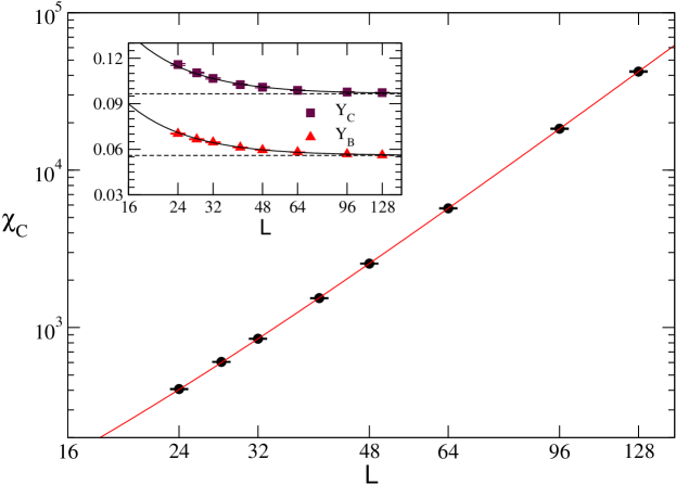
Figure 2: The inset shows $Y_{C}$ and $Y_{B}$ as a function of $L$ at $T=2.918$. We find $F^{2}=0.0965(5)$ and $B^{2}=0.0559(4)$. Using these values a fit of $\chi_{C}$ as a function of $L$ gives $\Sigma=0.2372(3)$ and $a=2.11(6)$ with a $\chi^{2}/DOF=0.5$. The main plot shows $\chi_{C}$ versus $L$ and the fit (solid line).

Figure 3 shows the dependence of $\chi_{C}$ as a function of $L$ for different temperatures. While $\chi_{C}$ increases as $L^{3}$ at $T=2.9275$, it saturates at $T=2.9285$ and $2.9292$ for large $L$. Note that extremely large lattices are necessary to see this saturation. Thus, there is a phase transition such that $2.9275<T_{c}<2.9285$. The peculiar non-monotonic behavior of $\chi_{C}$ before it saturates appears to rule out a second order behavior but is consistent with a first order transition. We can fit $\chi_{C}$ to the form

$$\chi_{C}=\frac{A+BL^{3}\exp(-\Delta FL^{3})}{1+C\exp(-\Delta FL^{3})}$$ (19)

which can be motivated as arising due to the presence of two phases whose free energy densities differ by $\Delta F$. We find this form captures the structure in the data well for $L\geq 48$ for both $T=2.9285$ and $2.9292$.

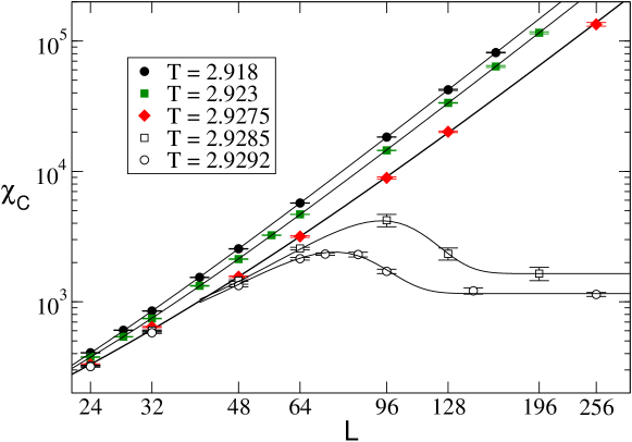
Figure 3: Plot of $\chi_{C}$ versus $L$ for different values of $T$ across the phase transition. The solid lines at $T=2.9285$ and $T=2.9292$ are fits to the first order form discussed in the text.

In the high temperature phase one can compute screening lengths $\xi$ by looking at the exponential decay of $G_{C}(z,z^{\prime})$ for large spatial separations between $z$ and $z^{\prime}$. Similarly in the low temperature phase $F^{2}$ and $B^{2}$ have dimensions of inverse length and hence can be used to provide natural length scales in the problem. At the phase transition we find that none of these length scales diverge but all are of the order of $40$ to $50$ lattice units indicating that the transition is a rather weak first order transition.

A renormalization group analysis of the fluctuations of the order parameter field, which in our case is a complex three vector field $\Phi_{i}(x),i=1,2,3$, has been performed using the $\epsilon$-expansion [26, 27]. Interestingly, the universal field theory one studies also describes the possible normal-to-planar super-fluid transition in ³He [28]. One finds no stable fixed point which implies that any observed phase transition must be a fluctuation driven first order transition. Our observations favor this conclusion. On the other hand recently it has been proposed that the $\epsilon$-expansion results may be misleading [28]. It is well known that first order transitions can arise due to model dependent features. In order to minimize such dependences it may be useful to repeat the above calculation for other values of $L_{t}$.

6.2 $d=3$ at zero temperature

In order to study zero temperature results we set $L_{t}=L$, $T=1$ and compute observables for various values of $\mu$ and $L$. In this case since $U_{B}(1)\otimes U_{\chi}(1)$ is expected to be broken completely the following should be observed:

• The diquark susceptibility $\chi_{B}$ should grow with the volume,

  $$\chi_{B}\sim\frac{\Delta^{2}}{2}L^{4}$$ (20)

  where $\Delta=\langle\chi_{1}\chi_{2}\rangle=\langle\overline{\chi}_{2}\overline{\chi}_{1}\rangle\neq 0$ is the diquark condensate.

• The chiral susceptibility $\chi_{C}$ should saturate with $L$ showing that the $G_{C}(z,z^{\prime})$ decays exponentially for large separations between $z$ and $z^{\prime}$. Note that the two correlators $G_{C}$ and $G_{B}$ are no longer related by a symmetry when $\mu\neq 0$.

• Both the helicity modulus $Y_{C}$ and $Y_{B}$, as defined in eqs.(12),(14) should grow linearly with $L$.

These expectations are borne out in our calculations as can be seen in Figure 4.

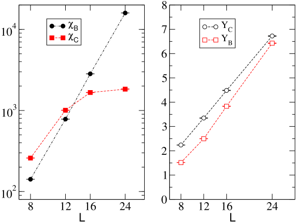
Figure 4: The left plot shows $\chi_{B}$ and $\chi_{C}$ as a function of $L$ at $\mu=0.01$. As expected $\chi_{B}$ grows as $L^{4}$ while $\chi_{C}$ saturates. For the same value of $\mu$ the right plot shows both $Y_{C}$ and $Y_{B}$ grow linearly with $L$.

As the chemical potential increases the lattice is filled with baryons. This can be seen in the inset of figure 5 where the baryon density is plotted as a function of $\mu$. Baryon super-fluidity cannot exist beyond saturation and this leads to a phase transition to the non-super-fluid phase. Renormalization group arguments show that this phase transition must belong to the mean field universality class for $d\geq 2$ [22]. It was recently shown that the critical chemical potential $\mu_{c}=0.5\cosh^{-1}(\sqrt{10})=0.909223..$ in the mean field approximation [16]. The diquark condensate was also shown to be

$$\Delta=\sqrt{\frac{1}{18}\left(\sqrt{10}-\cosh(2\mu)\right)}$$ (21)

In our calculations we extracted $\Delta$ by fitting $\chi_{B}$ to the relation

$$\chi_{B}=\frac{\Delta^{2}}{2}[L^{4}+AL^{2}+B].$$ (22)

Figure 5 shows our results along with the mean field result and the result with one-loop corrections. We find that $\mu_{c}$ is in excellent agreement with mean field theory while $\Delta$ requires the inclusion of one-loop corrections.

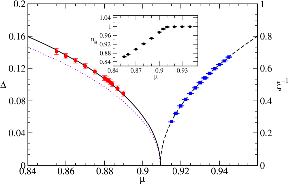
Figure 5: The plot of $\Delta$ and $\xi^{-1}$ as a function of $\mu$. The dotted line is the mean field result and the solid line includes the one loop corrections. The dashed line is a fit to the form $\xi^{-1}=A\sqrt{(\mu-\mu_{c})}$. The inset shows the baryon density $n_{B}$ as a function of $\mu$.

For $\mu>\mu_{c}$ it costs energy to remove a single baryon and we expect this energy to grow as $(\mu-\mu_{c})$. Since this phase describes non-relativistic particles the spatial correlation length $\xi$, obtained from $G_{B}(z,z^{\prime})$, must scale as $1/\sqrt{(\mu-\mu_{c})}$. Figure 5, also shows that this expectation is borne out.

6.3 $d=2$ Phase Diagram

We have also studied both the zero temperature and finite temperature phase transitions in two spatial dimensions. While the zero temperature transition is a mean field transition from a super-fluid phase to the saturated phase like in $d=3$, the finite temperature phase transition at $\mu=0$ is different and interesting. Mermin-Wagner theorem forbids the breaking of a continuous symmetry in $d=2$ at finite temperatures. However, the $U(1)$ part(s) of the $U(2)$ symmetry at $\mu=0$ can undergo a BKT type phase transition. This can result in long range correlations in $\chi_{C}$ and $\chi_{B}$ at low temperatures. If this is true one would expect

$$\lim_{L\rightarrow\infty}Y_{C}=\left\{\begin{array}[]{cc}\mathrm{Const.}&T<T_{c}\cr 0&T>T_{c}\end{array}\right.$$ (23)

while $\lim_{L\rightarrow\infty}Y_{B}=0$. Further, the screening lengths $\xi$ obtained from $G_{C}(z,z^{\prime})$ will behave as

$$\xi=A\exp\Bigg{(}\frac{B}{\sqrt{T-T_{c}}}\Bigg{)},\quad T>T_{c}$$ (24)

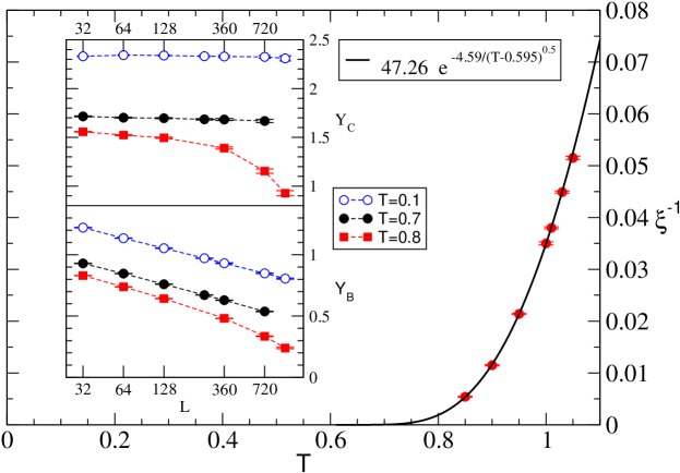
Figure 6:

Figure 6 shows that indeed our data is consistent with these expectations. We see that $Y_{C}$ is a constant and $Y_{B}$ decreases (although very slowly) with $L$ at $T=0.1$. For $T\geq 0.7$ we can begin to see both $Y_{C}$ and $Y_{B}$ decrease with $L$. For $0.8\leq T\leq 1.03$ $\xi$ extracted from $G_{C}(z,z^{\prime})$ fits well to the BKT form with $T_{c}\sim 0.6$. In a typical BKT phenomena, the super-fluid density is expected to show a universal jump at the transition. A naive estimate of this jump suggests that $Y_{C}(T=T_{C})=2/\pi\sim 0.6366...$, in our normalization. Our data shows a different jump suggesting that the transition is quantitatively different although qualitatively similar to the familiar BKT transition.

References

- [1] J. B. Kogut, M. A. Stephanov and D. Toublan, Phys. Lett. B 464, 183 (1999) [arXiv:hep-ph/9906346].
- [2] J. Wirstam, Phys. Rev. D 62, 045012 (2000) [arXiv:hep-ph/9912446].
- [3] C. Ratti and W. Weise, Phys. Rev. D 70, 054013 (2004) [arXiv:hep-ph/0406159].
- [4] J. T. Lenaghan, F. Sannino and K. Splittorff, Phys. Rev. D 65, 054002 (2002) [arXiv:hep-ph/0107099].
- [5] J. B. Kogut, J. Polonyi, H. W. Wyld and D. K. Sinclair, Nucl. Phys. B 265, 293 (1986).
- [6] J. B. Kogut, Nucl. Phys. B 290, 1 (1987).
- [7] O. Kaczmarek, F. Karsch and E. Laermann, Nucl. Phys. Proc. Suppl. 73, 441 (1999) [arXiv:hep-lat/9809059].
- [8] S. Hands, J. B. Kogut, M. P. Lombardo and S. E. Morrison, Nucl. Phys. B 558, 327 (1999) [arXiv:hep-lat/9902034].
- [9] S. Hands, I. Montvay, S. Morrison, M. Oevers, L. Scorzato and J. Skullerud, Eur. Phys. J. C 17, 285 (2000) [arXiv:hep-lat/0006018].
- [10] J. B. Kogut, D. K. Sinclair, S. J. Hands and S. E. Morrison, Phys. Rev. D 64, 094505 (2001) [arXiv:hep-lat/0105026].
- [11] J. B. Kogut, D. Toublan and D. K. Sinclair, Phys. Rev. D 68, 054507 (2003) [arXiv:hep-lat/0305003].
- [12] J. I. Skullerud, S. Ejiri, S. Hands and L. Scorzato, Prog. Theor. Phys. Suppl. 153, 60 (2004) [arXiv:hep-lat/0312002].
- [13] D. H. Adams and S. Chandrasekharan, Nucl. Phys. B 662, 220 (2003) [arXiv:hep-lat/0303003].
- [14] E. Dagotto, F. Karsch and A. Moreo, Phys. Lett. B 169, 421 (1986).
- [15] J. U. Klatke and K. H. Mutter, Nucl. Phys. B 342, 764 (1990).
- [16] Y. Nishida, K. Fukushima and T. Hatsuda, Phys. Rept. 398, 281 (2004) [arXiv:hep-ph/0306066].
- [17] G. Boyd, J. Fingberg, F. Karsch, L. Karkkainen and B. Petersson, Nucl. Phys. B 376, 199 (1992).
- [18] P. Rossi and U. Wolff, Nucl. Phys. B 248, 105 (1984).
- [19] U. Wolff, Phys. Lett. B 153, 92 (1985).
- [20] F. Karsch and K. H. Mutter, Nucl. Phys. B 313 541 (1989).
- [21] O.F. Syljuasen and A.W. Sandvik, Phys. Rev. E 66 046701 (2002).
- [22] M.P.A. Fisher, P.B. Weichman, G. Grinstein and D.S. Fisher, Phys. Rev. B40, 546 (1989).
- [23] G. V. Dunne and S. M. Nishigaki, Nucl. Phys. B 670, 307 (2003) [arXiv:hep-ph/0306220].
- [24] V.L. Berezinsky, Sov. Phys. JETP 34, 610 (1971); J.M.Kosterlitz and D.J. Thouless, J. Phys. C6 1181 (1973).
- [25] P. Hasenfratz and H. Leutwyler, Nucl. Phys. B 343, 241 (1990).
- [26] D.R.T. Jones, A. Love and M.A. Moore, J. Phys. C9, 743 (1976).
- [27] H. Kawamura, Phys. Rev. B38, 4916 (1988); erratum B42, 2610 (1990).
- [28] M. De Prato, A. Pelissetto, and E. Vicari, Phys. Rev. B 70, 214519 (2004).