Center Vortex Model for SU(3) Yang-Mills Theory

Abstract:

The center vortex model for the infrared sector of $SU(3)$ Yang-Mills theory is reviewed. After discussing the physical foundations underlying the model, some technical aspects of its realisation are discussed. The confining properties of the model are presented in some detail and compared to known results from full lattice Yang-Mills theory. Particular emphasis is put on the new phenomenon of vortex branching, which is instrumental in establishing first order behaviour of the $SU(3)$ phase transition. Finally, the vortex free energy is verified to furnish an order parameter for the deconfinement phase transition. It is shown to exhibit a weak discontinuity at the critical temperature, in agreement with predictions from lattice gauge theory.

PoS(LAT2005)320

1 Introduction

The vortex picture of the Yang-Mills vacuum was initially proposed as a possible mechanism of colour confinement. It is based on the idea that a random distribution of vortex colour flux is sufficient to effect an area law behaviour for large Wilson loops. Despite its simplicity and early successes [1], a precise confirmation of this scenario has been elusive for a long time. Recently, the picture has attracted renewed attention, mainly due to the advent of gauge fixing techniques which allow to detect center vortex structures directly within lattice configurations. Large-scale computer simulations have revealed ample evidence that the long-range properties of Yang-Mills theory can be accounted for in terms of vortices [2].

To complement the lattice approach, a random vortex world-surface model was introduced as an effective low-energy description of $SU(2)$ Yang-Mills theory [3]; it has recently been extended to the gauge groups $SU(3)$ [4, 5]. The fundamental assumption is that the long-range structure of Yang-Mills theory is dominated by thick, weakly interacting tubes of center flux which trace out closed surfaces in space-time. No analytical approach is known for such a quantum string ensemble. As a consequence, we realise our model on a space-time lattice with a fixed spacing $a$ to represent the transverse thickness of vortices. Short-distance structures smaller than $a$ (or, equivalently, momenta larger than $\pi/a$) cannot be resolved in this approach.

I will discuss the physical foundations of the center vortex model and some technical aspects in the next section. The main part of the talk is section 3 which presents a selection of results obtained in the model. In Section 4, I conclude with a brief summary and some general comments.

2 Phase diagram and choice of parameters

Vortices are closed lines of colour flux in three space dimensions and, correspondingly, closed world-surfaces in space-time. Their dimensionality is unique in that they can have a topologically stable linking with Wilson loops. The colour flux placed on the vortex is quantized such that each linking with a Wilson loop $W(\mathscr{C})$ (i.e. each intersection point of the closed loop $\mathscr{C}$ with the vortex surface) contributes a center element of $SU(N)$ to $\langle W(\mathscr{C})\rangle$. To describe such intersections, the vortex surface must be defined on a lattice which is dual to the one where Wilson loops (and gauge connections) live. This emphasises the dual character of our model.

Technically, we create random vortex surfaces on the dual lattice by assigning triality to the elementary squares. The fixed lattice spacing $a$ defines the minimal distance at which two intersection points can be resolved, i.e. the thickness of the vortex tube or sheet. Random surfaces created in this way are weighted by a model action containing a Nambu-Goto and a curvature term [4], symbolically

$$S=\sum_{\rm plaq}\epsilon\,\,\,\begin{minipage}{42.67912pt}\includegraphics[width=42.67912pt]{plaq.eps} \end{minipage}+\frac{c}{2}\quad\begin{minipage}{42.67912pt} \includegraphics[width=42.67912pt]{bend.eps} \end{minipage}$$ (1)

The parameters are determined by measuring the zero-temperature string tension $\sigma_{0}$ (in units of the lattice spacing). One observes a deconfined region at large couplings $(\epsilon,c)$ with a shallow cross-over to a confined region at small $(\epsilon,c)$ [4]. In the latter domain, one can also effect a deconfinement phase transition by increasing the temperature of the simulation (i.e. by reducing the temporal lattice extension). Using an interpolation procedure, the ratio of the critical temperature, $T_{c}$, to the zero-temperature string tension, $\sigma_{0}$, can be extracted at all couplings. Comparision with the known value $T_{c}/\sqrt{\sigma_{0}}=0.63$ from $SU(3)$ lattice gauge theory then yields a line of possible physical values in parameter $(\epsilon,c)$ space. As it turns out, the long-range physics are almost constant on this parameter line so that we are free to make the arbitrary choice,

$$\epsilon=0\,,\qquad c=0.21\,.$$ (2)

From the string tension $\sigma_{0}\,a^{2}$ measured at this point, the overall scale can be determined using the phenomenological value $\sigma_{0}=(440\,\mathrm{MeV})^{2}$ from QCD. This gives a vortex thickness of $a=0.39\,\mathrm{fm}$.

3 Applications

Figure 1: String tension between two static colour charges (crosses) and spatial string tension (squares) as a function of temperature. Measurements were taken on a $16^{3}\times N_{0}$ lattice for the physical choice of parameters eq. (2.2).

3.1 Spatial string tension

The zero-temperature string-tension $\sigma_{0}$ used to fix the parameters is extracted from Wilson loops extending in one space and the time direction. In addition, purely spatial Wilson loops can also be measured, although they do not have an immediate interpretation as an inter-quark potential. From lattice gauge theory, it is known that spatial Wilson loops exhibit an area law at all temperatures and the spatial string tension extracted from them persists in the high-temperature phase [6]. As shown in fig. 1, our model reproduces this strongly correlated hot phase; in fact, our results for the spatial string tension agree with ref. [6] to within $5\%$. This success can be attributed to the percolation behaviour of vortex clusters.

3.2 Finite temperature phase transition and vortex branching

The confinement mechanism is most clearly seen in the details of the phase transition at non-zero temperatures. Histograms of the action density measured at the critical temperature reveal a qualitative difference between the gauge groups $SU(2)$ and $SU(3)$: The $SU(3)$ transition exhibits the shallow double-peak structure characteristic for a weak first order transition, while the $SU(2)$ transition is continuous (second order) [4]. This pattern is also seen in full lattice gauge theory.

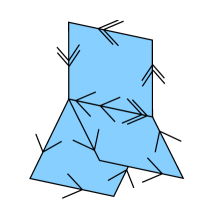
Figure 2: The right-hand panel displays a four-dimensional lattice view, where a vortex surface, consisting of elementary squares, branches along a $\nu=3$ bond. The left panel shows the same situation projected to a 3D slice.

To understand the origin of this difference, we have to look at the vortex geometry in more detail. In $D=4$ dimensions, each bond on the dual lattice is attached to six elementary squares, which are assigned trialities $q\in\{0,1,2\}$ in our model. The local geometry of a world surface is then characterised by the number $\nu=0,\ldots,6$ of vortex surfaces ($q\neq 0$) meeting at a given bond. The odd values $\nu=3,5$ are not allowed in $SU(2)$ and represent genuine $SU(3)$ vortex branchings, cf. fig. 2. Note that the triality $q=1,2$ of a vortex square can be reversed by flipping its orientation; moreover, triality is only conserved modulo 3 and a Dirac string ($q=3$) may be added to any configuration. The branching in fig. 2 is thus equivalent to a situation where three $q=1$ vortices emerge from a common point (or bond in $D=4$). Branching lines in $D=4$ are therefore similar to center monopole worldlines.

The statistical distribution of branchings is best studied in 3D slices of the lattice, whence possible branching bonds are projected onto points of type $\nu$. From fig. 3, we conclude that the largest volume fraction in the confined phase corresponds to non-branching vortex matter ($\nu=2$), with a considerable probabitlity of both self-intersection ($\nu=4,6$) and genuine branchings ($\nu=3,5$). Only $15\%$ of the volume is not occupied by vortices ($\nu=0$). In the deconfined phase ($T>T_{c}$), the situation is qualitatively unchanged for time-slices, while space-slices show virtually zero branchings above $T_{c}$. This can be understood if the vortices undergo a (de)percolation phase transition for $T>T_{c}$ and most vortex clusters wind directly around the short time direction [4]. The same phenomenon explains the persistence of the spatial string tension discussed above.

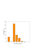
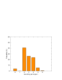
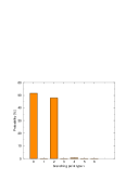
Figure 3: Volume fractions occupied by points of a certain branching type $\nu$ within $3D$ lattice slices. The left panel shows the distribution at zero temperature in the confined phase. The middle and right panel both correspond to $T>T_{c}$, with the middle referring to a time slice and the right to a space slice.

3.3 Vortex free energy and the ’t Hooft loop

The ’t Hooft loop can be viewed as a creation operator for (quantized) flux along a closed spatial line $\mathscr{C}$. It was formally introduced by ’t Hooft in 1978 as a dual order parameter for the deconfinement transition on a space-time torus. Recently, explicit realisations of this construction have been given both in the continuum [7] and on the lattice [8], where maximally extended ’t Hooft loops implement twisted boundary conditions.

In the center vortex model, the ’t Hooft loop is literally an (open) vortex creation operator [5]: Its action is to add a fixed triality $q=1,2$ to each elementary square in a world-sheet over $\mathscr{C}$; since triality is additive, this simply injects a center vortex of type $q=1,2$ in the current configuration. The exact form of the world-sheet over $\mathscr{C}$ is irrelevant (and center-gauge dependent), but for simplicity, we restrict ourselves to planar loops $\mathscr{C}$ and minimal surface sheets over them.

The action penalty $\Delta S$ incurred by the vortex creation is related to the vortex free energy $F$ via $e^{-F}=\langle e^{-\Delta S}\rangle$. As mentioned above, the free energy is expected to furnish an order parameter for the deconfinement transition with essentially the opposite behaviour as the Wilson loop. This is nicely confirmed in our model: The left panel of fig. 4 exhibits a linear rise of the free energy with the area of the ’t Hooft loop at $T>T_{c}$, which allows to define a dual string tension $\sigma_{D}$ in the deconfined phase.

As we approach the phase transition from above, the dual string tension quickly vanishes (cf. right panel of fig. 4). In the confined phase, the subleading perimeter law is hidden in the statistical noise, and the vortex free energy is consistent with zero (vortex condensation). Precise measurements close to the transition reveal a small discontinuity

$$\left.\sqrt{\sigma_{D}}\right|_{T=T_{c}+}=(34.5\pm 4.9)\,\mathrm{MeV}$$ (3)

in the free energy, which should be compared to the ordinary zero-temperature string tension $\sigma_{0}=(440\,\mathrm{MeV})^{2}$ setting the overall scale. This demonstrates again the weakness of the first order transition for the colour group $G=SU(3)$. Quantitatively, our findings are in fair agreement with lattice caluclations [8] which seem to favour a slightly larger value $\sigma_{D}\simeq(48\,\mathrm{MeV})^{2}$.

         

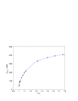
Figure 4: Left Panel: Free energy of ’t Hooft loops in the deconfined phase ($T/T_{c}=1.093$), as a function of the minimal area over the loop. Right panel: The dual string tension $\sigma_{D}$ as a function of the temperature. Measurements were performed on a large $30^{3}\times N_{0}$ lattice with $N_{0}=1,2$.

4 Further remarks and conclusions

In this talk I have presented an effective model for the infra-red sector of $SU(3)$ Yang Mills theory, based on random world surfaces carrying center flux. Assuming only that vortex sheets have a surface tension and stiffness, the model reproduces many non-trivial properties of long-range Yang-Mills theory. Among the examples discussed here are the spatial string tension, the order and strength of the phase transition for various gauge groups, and the discontinuity of the vortex free energy across the $SU(3)$ phase transition.

The geometrical structure of vortex branchings is the key property in establishing first order behaviour for the $SU(3)$ model. Geometry alone, however, is not sufficient to determine the physics of a vortex model; the effective vortex dynamics specific to each gauge group play a crucial role. In principle, the vortex dynamics would be determined by integrating out all non-vortex degrees of freedom; our project is essentially the reverse approach of guessing a model action and comparing to low-energy Yang-Mills theory.

For $SU(3)$, the results indicate that the simple two-operator action, eq. (1), is sufficient. With increasing complexity of the colour group, however, additional terms may arise which favour vortex branchings (center monopoles) explicitly; such terms tend to enhance the strength of the phase transition. In fact, preliminary investigations for $G=SU(4)$ indicate that such terms are indeed necessary and may become even more pronounced with increasing number of colours.

References

-
[1]
G. ’t Hooft, Nucl. Phys. B138 (1978) 1;
G. Mack, V. B. Petkova, Ann. Phys. (NY) 125 (1980) 117;
J. M. Cornwall, Nucl. Phys. B157 (1979) 392;
H. B. Nielsen, P. Olesen, Nucl. Phys. B160 (1979) 380. -
[2]
J. Greensite, Prog. Part. Nucl. Phys. 51 (2003) 1
[hep-lat/0301023], and references therein;
K. Landfeld, H. Reinhardt, O. Tennert, Phys. Lett. B419 (1998) 317 [hep-lat/9710068];
M. Faber, J. Greensite, S. Olejnik, Phys. Lett. B474 (2000) 177 [hep-lat/9911006];
P. de Forcrand, M. D’Elia, Phys. Rev. Lett. 82 (1999) 4582 [hep-lat/9901020]. - [3] M. Engelhardt, H. Reinhardt, Nucl. Phys. 585 (2000) 591 [hep-lat/9912003].
- [4] M. Engelhardt, M. Quandt, H. Reinhardt, Nucl. Phys. B685 (2004) 227 [hep-lat/0311029].
- [5] M. Quandt, H. Reinhardt, M. Engelhardt, Phys. Rev. D71 (2005) 054026 [hep-lat/0412033].
- [6] G. Boyd et al., Nucl. Phys. B469 (1996) 419 [hep-lat/9602007].
- [7] H. Reinhardt, Phys. Lett. B557 (2003) 317 [hep-th/0212264].
-
[8]
P. de Forcrand, M. D’Elia, M. Pepe, Phys. Rev. Lett. 86
(2001) 1438 [hep-lat/0007034];
P. de Forcrand, L. Smekal, Phys. Rev. D66 (2002) 011504 [hep-lat/0107018].