Performance of machines for lattice QCD simulations

Abstract:

We review the architecture of massively parallel machines used for lattice QCD simulations and present benchmarks for the performance of popular algorithms on these platforms. We cover commercial supercomputers, PC clusters, and custom-designed machines. We also speculate on future developments.

PoS(LAT2005)019

1 Introduction

Lattice gauge theory is a rather mature field of research. There are many well-defined questions, of both fundamental and phenomenological importance, to which we can obtain definite answers provided sufficient computing power is available. While steady progress has been made on the theoretical and algorithmic fronts, advances in computing technology have probably made the largest contribution to the performance increase of lattice QCD simulations in the past. This is likely to remain the case in the future.

Clearly, the computational demands of large-scale lattice QCD simulations [1] can only be satisfied by massively parallel machines. There are many considerations contributing to the design (or purchase) and the operation of such a machine, most of which will be discussed in this review. From a funding agency’s point of view, leaving aside political and other nontechnical issues, the bottom line is the cost-effectiveness of the machine, i.e., the “science output” per unit of currency. All other details being equal, such as the particular physical quantity to be computed and the algorithm employed, a good measure for this is the sustained performance (to be defined below) of a parallel machine per unit of currency. Of course, things are not as simple as a single number, and one of the purposes of this paper is to elucidate some of the important details that are hidden behind such a number.

The structure of this paper is as follows. In Sec. 2, we introduce some basic aspects of parallel computing to make the presentation accessible to the non-expert reader. We then summarize performance-relevant issues that play a role in the design of parallel machines in Sec. 3. This is followed by the main part of the paper, Sec. 4, in which we introduce popular machine architectures used by the lattice community (commercial supercomputers, PC clusters, and custom-designed machines) and present benchmarks for the performance of lattice QCD algorithms on these platforms. Section 5 speculates on future developments, and conclusions are drawn in Sec. 6.

Lattice QCD practitioners are not only expert users of massively parallel machines, they are also actively involved in the design and development of new parallel computing technology, both in the hardware and in the software sector. There is enormous talent, expertise, and experience available in our community (which, unfortunately, is typically operating under rather tight financial constraints). This review is in large part a reflection of the hard and ingenious work of these researchers.

2 Parallel computing basics

In general, parallelization of a computational task means the distribution of various parts of this task onto several resources. Parallelism can be exploited at several levels. For example, modern CPUs utilize the so-called instruction-level parallelism of a program by pipelining the various stages of an instruction and executing them in parallel. In a more restricted sense, we often use the term parallelization to mean the numerical solution of a problem on several processors, with each processor working on a subvolume of the problem. These processors need to communicate through some sort of interconnection network. Lattice QCD is particularly amenable to this kind of parallelization since (a) one typically uses a regular hypercubic grid that can easily be split into identical subvolumes, (b) the boundary conditions are simple, and (c) the communication patterns between compute nodes are uniform and predictable. For example, a state-of-the-art simulation with dynamical fermions on a $32^{3}\times 64$ global volume could be done on a parallel machine with 8,192 nodes and a local (i.e., per-node) volume of $4^{4}$. Since the same program is executed on all nodes, the machine is said to operate in SPMD (single program, multiple data) mode.

The performance of a parallel machine depends on the performance of its hardware components (processor, memory susbsytem, and communications network) and on the software that runs on the machine (application code, libraries, operating system). The overall performance can be quantified in terms of peak and sustained performance. The peak performance is a single number that is simply the number of processors (which we assume to be identical) times the peak performance of a single processor. The latter is the product of the clock frequency and the number of double-precision floating point operations (Flops) that can be executed in a single clock cycle. For example, a cluster of 256 Pentium-4 PCs (two Flops per cycle) running at 3 GHz has a peak performance of 1.5 TFlop/s. What really matters, of course, is the sustained performance, which is the actual number of Flops executed (on average) by the application code per clock cycle, again multiplied by the clock frequency and the number of processors. The sustained performance is often quoted as percentage of peak, which gives an indication of how well a particular application performs on a given machine. However, as mentioned above, it is the sustained performance in Flop/s per unit of currency that is the best measure of the cost-effectiveness of a machine.

We can now think of defining a “cost-effectiveness function” that depends on several control parameters which we can tune to maximize this function. Examples of such control parameters are

• clock frequency,

• number of Flops per clock cycle (e.g., SIMD vector operations),

• number of processors,

• percentage of peak sustainable,

• expenses for power, cooling and floor space.
  

Of course, there are dependencies between these parameters, e.g., a higher frequency in general means higher power consumption, and a larger number of processors often means smaller sustained performance because more communication is needed. The most interesting and nontrivial parameter is clearly the sustained performance on which we will mainly focus in the following. It depends on a variety of factors such as

• stalls due to memory access (if the data are not in cache),

• stalls due to communication between processors,

• software overhead, e.g., for operating system or communication calls,

• imbalance of multiply and add in the algorithm (e.g., some CPUs such as PowerPC and Itanium provide so-called fused multiply-add, or FMA, instructions, and if the numbers of multiplies and adds differ, the peak performance cannot even be obtained in theory).
  

Clearly, hardware and software should be designed or selected to minimize the dead time and to maximize the sustained performance. There are many details that need to be taken into account, but the final result can be exhibited in a rather simple way in a so-called scalability plot, where the sustained performance is plotted as a function of the number of processors participating in the calculation. Such a plot contains the essential information about the quality of a machine. However, two kinds of scalability plots need to be distinguished:

• “weak scaling”: Here the local volume is kept fixed, and thus the global volume, i.e., the problem size, increases linearly with the number of processors.

• “strong scaling”: Here the global volume is kept fixed so that the local volume decreases with the number of processors.
  

The latter case is the more interesting one since we typically want to solve a fixed physical problem in the shortest possible wall clock time. (To give a simple example from another field, the weather forecast for tomorrow better be done by today.) Ideally, one would like to obtain linear scaling, i.e., a linear increase of the sustained performance with the number of processors. However, a decreasing local volume results in two competing effects: (1) more (or even all) of the data associated with the local subvolume will fit in cache (or on-chip memory), which is good, and (2) the surface-to-volume ratio of the local subvolume increases, which is bad, since more communication needs to be done per unit of computation (the communication effort typically increases with the surface area, whereas the computing effort typically increases with the volume). In the fortunate case that effect (1) is dominant, one would observe superlinear scaling. More typically, effect (2) dominates, leading to sublinear scaling or even saturation.

A large part of the effort in designing a massively parallel machine is directed at suppressing, or at least partially evading, the consequences of effect (2). The corresponding techniques are known as “communications latency hiding”. To understand this better, we remind the reader of two basic parameters characterizing a network connection, i.e., bandwidth and latency, shown schematically in Fig. 1.

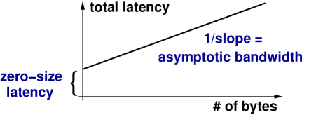
Figure 1: In a simple model of network performance, the time (or total latency) it takes to transfer a packet of a certain size depends on the zero-size latency (which includes sender and receiver overhead as well as time of flight) and on the asymptotic (or maximum) bandwidth of the network: total latency = zero-size latency + (# of bytes)/(asymptotic bandwidth). Sometimes people quote the actual bandwidth (or throughput), defined as (# of bytes)/(total latency). For large packet size this converges to the asymptotic bandwidth.

(In the remainder of this paper, we will use the terms latency and bandwidth to denote the zero-size latency and the asymptotic bandwidth, respectively, unless stated otherwise.) If a large number of bytes needs to be transfered, bandwidth is the more important factor since the latency only makes a small contribution to the total transmission time. However, for small packets, latency is the dominant part of the total time. This is the relevant case when the local volume becomes small, as it does in the case of strong scaling, since the amount of information that needs to be communicated to another node, and therefore the packet size, is small. (A simple example is provided by ping times in online gaming: the amount of information to be transmitted, e.g., the target coordinates of the enemy, is small, and thus the success of the gamer critically depends on small latencies, i.e., short ping times.) The term communications latency hiding refers to techniques in which computation and communication are overlapped, i.e., the CPU can do useful computations while the communication is in progress.

Various aspects of network performance can be measured in special benchmarks. For example, the classic measure of latency and bandwidth is a “ping-pong” benchmark in which a single message is bounced back and forth between two nodes. In a “ping-ping” benchmark, two messages are bounced back and forth in both directions simultaneously, and the measured performance gives an indication of the interference between opposite directions (which can be due to hard- and/or software reasons).

We close this section by introducing the concept of capability and capacity machines. Roughly speaking, capability is the ability of a machine to finish a given (typically very difficult) calculation in a certain amount of time, whereas capacity refers to the ability of a machine to carry out a given workload (typically consisting of many jobs) in a certain amount of time. A given machine has both attributes, but one often speaks of capability machines (if the sustained performance remains high in the strong-scaling case) and of capacity machines (which only scale weakly). In lattice QCD, both types of machine are used. Capability machines are needed to generate dynamical configurations with small quark masses in a single Markov chain. Capacity machines are suitable for most analysis tasks and for scans of parameter space.

3 Design considerations

There are essentially three possibilities to obtain a massively parallel machine: one can purchase a commercial supercomputer, one can build a machine out of commercial off-the-shelf (COTS) components, or one can custom-design a machine. In all of these cases, the considerations that play a role in the design or purchase process are similar. They naturally fall into two categories, hardware and software, which we shall discuss in this section. Most importantly, the design should be balanced in the sense that there are no bottlenecks. It does not make sense to spend money or design efforts on a high-performance component which is then slowed down by other components that cannot keep up with it.

Of course, the machine should be designed or selected such that lattice QCD applications perform well on it. The workhorse in dynamical-fermions simulations is the conjugate gradient (CG) inversion algorithm and variants thereof. Its main two ingredients are (a) (sparse matrix)$\times$vector multiplication and (b) global sums. Therefore the benchmarks presented in Sec. 4 will concentrate on these two operations and on the overall performance of the CG inverter for various Dirac operators. (For an earlier set of benchmarks presented at LATTICE 2003, see Ref. [2].)

On the hardware side, attention should be paid to the following points.

• Processor. This is the heart of the machine. It should have high peak performance, a large amount of cache or on-chip memory, and fast interfaces to external memory and the network. It should be programmable in one or more standard languages, and high-quality compilers should be available for it. Lattice QCD code should obtain high sustained performance on a single node.

• Memory system. In addition to on-chip memory, each node should have a sufficient amount of external memory that can be accessed with low latency and high bandwidth. On a small machine, the memory might be shared, i.e., all nodes can access a common memory. On a very large machine, the memory will be distributed, i.e., the nodes need to send messages to exchange data. Some machines provide a mixture of shared memory (on subpartitions of the machine) and distributed memory, see, e.g., Sec. 4.1.1. In all cases, cache coherence should be guaranteed in hardware.

• Network. As stated above, the network should enable packet transfers with low latency and high bandwidth. As much of the latency as possible should be hidden, e.g., by direct memory access (DMA) hardware that can unburden the CPU. Also, hardware acceleration for critical operations (such as global sums) could be included in a custom-designed machine. The topology of the network also plays an important role. Switched networks typically suffer from higher latencies, whereas mesh-based networks require more cables. Finally, there should be sufficient bandwidth for I/O to disk.

• Other issues. Obviously, the price of the various components enters the above mentioned cost-effectiveness function. Expenses for power and cooling need to be taken into account. The packaging density (which, incidentally, may affect the network performance through cable lengths) and the resulting footprint of the machine may be an issue if space is restricted. Last but not least, the machine should be reliable and easy to maintain.
  

On the software side, several factors come into play.

• Operating system (OS). It should provide all necessary services without hindering performance. Often the best solution is a single-user, single-process OS.

• Compilers. If standard languages such as C/C++ or Fortran are supported, compilers should be available that produce correct and efficient code. Ideally, they should be free as well (Gnu tools). In addition, automatic assembler generators such as BAGEL [3] are desirable to increase the code performance without undue burden on the programmer.

• System libraries. Communication calls and other important functions such as parallel I/O are typically implemented in system libraries. For example, on machines with distributed memory, the MPI (message-passing interface) library is often used to send messages, whereas on shared-memory machines, the OpenMP library can be employed to specify shared-memory parallelism. It is important that these libraries be implemented efficiently, making use of the hardware features specific to the machine.

• Application code. There are many code systems in use in the lattice QCD community, some of which are freely available [4, 5, 6, 7]. Such a code system should be easy to understand, easy to use, and easy to extend. It should also be portable to as many popular architectures as possible. Of course, it should also provide high performance, which can be achieved by the use of optimized kernels for critical code sections (often in assembler).
  

Regarding the last two points, the efforts of the USQCD software team and their collaborators [8] to create and maintain a portable and efficient software system for lattice QCD deserve special mention.

4 Parallel architectures used for lattice QCD

In this section, we describe a representative subset of the parallel architectures used for lattice QCD simulations, including benchmarks and cost-effectiveness. Since our emphasis is on parallel computing, we shall not discuss single-node performance in detail. On all of the machines discussed below, the critical kernels have been optimized in assembler (including clever cache management) and obtain single-node performance close to the theoretical maximum.

Also, we will not address the issue of reliability in detail because reliable numbers beyond rough estimates or anecdotal evidence are hard to come by. All of the machines discussed below are reliable in the sense that the mean time between failures is longer than typical checkpointing intervals.

A note of warning: when computing the cost-effectiveness of a particular architecture, a factor of two can pop up if, as in the case of PC clusters, single-precision calculations are a factor of two faster than in double precision. Whether or not double precision is really necessary depends on the application, and in many cases one can certainly get by with a mixture of mainly single and some double precision. Having said this, the numbers quoted below are all based on double precision unless stated otherwise.

4.1 Commercial supercomputers

Commercial machines are available from a variety of vendors such as IBM, Cray, Hitachi, SGI, and others. Typically, they are designed to obtain reasonable sustained performance for a wide range of applications. This implies that their architecture is not necessarily optimal for lattice QCD. Furthermore, they are typically rather expensive and can therefore be found mainly in large national or regional computing centers where the lattice community can only get a fraction of the computing time. Nevertheless, they provide a non-negligible fraction of the total computing power available to our community and are particularly useful when employed as capacity machines.

We have chosen to concentrate on two machines that will be used for lattice QCD simulations in the next few years, the SGI Altix and IBM’s BlueGene/L. For the performance of lattice QCD code on the Earth Simulator, see Ref. [9].

4.1.1 SGI Altix

The SGI Altix is based on the Intel Itanium 2 processor. This is a 64-bit processor based on the so-called EPIC (explicitly parallel instruction computing) architecture, which in turn is an enhancement of the VLIW (very long instruction word) concept. The basic idea here is for the compiler to group independent machine instructions in so-called bundles which can then be executed in a single clock cycle. This results in simpler hardware than in the case of a superscalar RISC CPU, where the burden of recognizing dependencies and scheduling instructions dynamically lies with the hardware. Clearly, the quality of the compiler, i.e., its ability to parallelize instructions statically, is of utmost importance for the performance of the Itanium architecture.

The architecture of the Altix is shown schematically in Fig. 2.

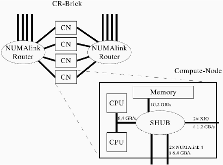
Figure 2: Main components of the SGI Altix system. Figure taken from Ref. [10].

A compute node consists of two (single- or dual-core) CPUs that are connected to local memory, to the network, and to I/O devices via a custom-designed super-hub (SHUB) chip. The maximum attainable bandwidths are shown in Fig. 2. An obvious disadvantage of this design is contention for memory and network accesses; however, this is partially mitigated by the large cache size of the Itanium 2 (up to 9 MB).

The network of the Altix uses the ccNUMA (cache coherent non-uniform memory access) architecture and is called NUMAlink. Four compute nodes are connected to form a compute-router (CR) brick by NUMAlink routers in a fat-tree topology, as shown in Fig. 2. A fat tree of CR bricks can then be built using first- and second-level NUMAlink routers. The MPI latency of NUMAlink4 is claimed to be 1 $\upmu$s, to which each hop across a router adds roughly 50 ns. A distinguishing feature of the Altix is the possibility of a shared-memory domain with up to 512 CPUs.

The only lattice QCD benchmarks available so far are weak-scaling studies of applications of the Wilson Dirac operator (Wilson Dslash in short), i.e., the matrix$\times$vector component of the CG algorithm. These benchmarks were performed by Thomas Streuer on the 64-node test system in Munich, see Table 1. Note that the local volume is so small that the problem fits in L3 cache. All communications were done using shared memory (shmem_put), and hand-coded assembler was used to obtain the quoted numbers.

# CPUs	$V_{\text{global}}$	sustained perf.
8	$8^{3}\times 4$	31%
16	$8^{4}$	26%
32	$8^{3}\times 16$	30%
64	$8^{3}\times 32$	28%

Table 1: Performance of the Wilson Dslash on the SGI Altix. In all cases, $V_{\text{local}}=4^{4}$.

The performance is quite impressive, but it remains to be seen how it scales as the global sums are included and as the number of nodes is increased, once the full machine is available.

At the Leibniz Computing Center in Munich, a system with 33 TFlop/s peak (2,560 1.6 GHz dual-core Montecito sockets with 6 MB L3 cache each and 20 TB of main memory) will be operational at the beginning of 2006, and an upgrade to 69 TFlop/s peak (3,328 2.6 GHz dual-core Montvale sockets with 9 MB L3 cache each and 40 TB of main memory) will occur in 2007. The purchase price for this system is 38 million Euro, not including substantial running costs. Assuming that the performance numbers quoted in Table 1 go down on larger machines by a factor of two or so, and figuring in the additional cost of global sums, an optimistic estimate for the cost-effectiveness of this particular machine for lattice QCD is thus on the order of 5 Euro per sustained MFlop/s in 2007, i.e., two years from now. As we shall see, this is substantially more expensive than the 2005 numbers for the other machines to be discussed below.

4.1.2 BlueGene/L

IBM’s flagship supercomputer, BlueGene/L (BG/L in short), currently occupies the No. 1 and 2 spots on the Top 500 list (183 TFlop/s peak at LLNL and 115 TFlop/s peak at IBM Watson). Its design has been influenced by, and is similar to, that of QCDOC (and QCDOC’s predecessor, QCDSP), see Sec. 4.3.2 below.

The architecture of BG/L has been described in detail in Ref. [11], the performance of lattice QCD code was addressed in Ref. [12], and an entire journal issue was dedicated to BG/L in Ref. [13]. We briefly summarize the relevant points here. The heart of the machine is an application-specific integrated circuit (ASIC) containing two 700 MHz PowerPC 440 CPU cores to each of which are attached two 64-bit FPUs that can be utilized to execute two FMA instructions per clock cycle. The peak performance of a single ASIC is thus 5.6 GFlop/s. There is a shared 4 MB L3 cache on chip, and external memory is distributed, with 512 MB per node. The nodes are connected in a three-dimensional torus with nearest-neighbor connections (but without DMA capabilities). In addition, there is a global tree network that is used for global reductions.

BG/L can be run in one of two modes.

• Co-processor mode. One of the 440 cores is used for computation, the other one for communication. Thus, the peak performance is cut in half to 2.8 GFlop/s.

• Virtual-node mode. Both of the 440 cores are used for computation and communication. The peak performance is now the full 5.6 GFlop/s, but computation and communication cannot be overlapped.
  

Which of these two modes results in higher sustained performance depends on the application. The performance numbers quoted in Ref. [12], and reproduced in Fig. 3 for convenience, were obtained in virtual-node mode using C/C++ inline assembler and carefully tuned code that takes advantage of special hardware features of BlueGene/L.

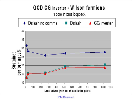
Figure 3: Strong scaling of Wilson Dslash and CG on BlueGene/L [12]. Source: Pavlos Vranas.

Although the numbers in Fig. 3 were obtained on only one node (i.e., two cores), the performance estimates are realistic since the torus network was used for the communications. A weak-scaling benchmark of the Wilson CG (using a local volume of $4^{3}\times 16$) showed a very mild degradation of the sustained performance as the number of nodes was increased [12]. This was most likely due to the fact that the global sums were done on the torus instead of the global tree network because the necessary software was not yet available at the time. They can now be done on the global tree, so the degradation should disappear.

For reasons unbeknownst to the author, the groups that bought a BG/L machine are not allowed to disclose the purchase price. Of course, rumors abound, and for the sake of argument we will estimate the price to be $2 million per rack. A rack consists of 1,024 nodes, thus the sustained performance of a large-scale lattice QCD application (assuming, say, 17% of peak) is on the order of 1 TFlop/s per rack, which translates into a cost-effectiveness of about $2 per MFlop/s.

4.2 PC clusters

PC clusters have been reviewed at previous LATTICE conferences [14, 15] and were presented this year as well [16]. Clearly, they are a sensible choice for many (lattice and non-lattice) groups. The high-volume market for PCs drives down the cost of the components so that small- or medium-size clusters can be obtained by groups that do not have access to multi-million dollar funding. Also, the software running on PC clusters is reasonably standard and can be used with relatively modest effort.

In the sub-TFlop/s range, PC clusters are probably the best overall choice in terms of cost-effectiveness and ease of use. The main question is whether the available networking components allow PC clusters to scale beyond this performance at a price competitive with the custom-designed machines discussed in Sec. 4.3 below. This is the point on which we will try to shed some light. Note, however, that PC clusters are very much a moving target since new hardware appears on the market all the time. Consequently, we can only provide a snapshot of the current status. For more details, we refer to Refs. [17, 18]. The currently installed lattice QCD clusters with a peak performance of more than 1 TFlop/s are summarized in Table 2.

Name	Institution	CPU	Network	Peak (TFlop/s)
ALICEnext	Wuppertal	1024 Opteron	Gig-E (2d mesh)	3.7
4G	JLAB	384 Xeon	Gig-E (5d mesh)	2.2
3G	JLAB	256 Xeon	Gig-E (3d mesh)	1.4
Pion	Fermilab	260 (520) P4-640	Infiniband	1.7 (3.4)
W	Fermilab	256 P4E-Xeon	Myrinet	1.2

Table 2: Existing lattice QCD clusters with more than 1 TFlop/s peak performance (double precision). The Pion numbers in parentheses refer to a planned expansion in the fall of 2005.

The hardware components making up a PC cluster can be roughly divided into CPU, memory system, and network (including I/O interface), which we shall discuss in turn. Of the currently popular processors, Intel’s Pentium 4 and Xeon as well as AMD’s Opteron appear to offer the best price-performance ratio. The difference between the P4 and the Xeon is that the former is strictly a uniprocessor whereas the latter is capable of symmetric multi-processing (SMP). The Opteron has the advantage of having the memory controller on chip, but it tends to be a little pricier. Since most of the available benchmarks were obtained with Intel CPUs, we will concentrate on these chips. While there are some differences between the various processors on the market, the issues that arise in terms of cluster building are very similar for all of them, so the conclusions we will draw are universal.

Clock frequencies nowadays are approaching 4 GHz so that the peak performance of a single processor is getting close to 8 GFlop/s. Using the SIMD graphics vector extensions provided by Intel and AMD processors [19, 20], lattice QCD code can obtain 50% or more of peak when operating from cache [21, 15], see Fig. 4 for a typical benchmark.

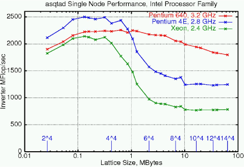
Figure 4: Single-node performance of the asqtad inverter (in single precision) on various Intel CPUs. Cache size and frequency of the front-side bus are as follows. Xeon: 0.5 MB, 400 MHz; P4E: 1.0 MB, 800 MHz, P640: 2.0 MB, 800 MHz. From Ref. [18].

Once the problem moves out of cache, the performance is no longer limited by the floating-point capabilities of the processor but by the performance of the memory bus. This can also be seen in Fig. 4. Thus, if a physics problem is to be solved on a small cluster, where the local volume tends to be large, the memory bus is likely to be the bottleneck. On a larger cluster, where the local volume might fit in cache, the bottleneck moves to the network interface.

While newer processors typically come with a faster memory bus for little or no extra money, the cost of better networking components can represent a significant fraction (perhaps one half) of the total expense for a PC cluster. The relevant parameters are latency and bandwidth, and the topology of the network plays a role as well. Mesh-based networks with nearest-neighbor connections are well-suited for lattice QCD and are quite cheap since switches are not necessary; however, they require more cables, are less fault-tolerant, and accumulate latencies when computing global sums. Switched networks provide all-to-all communication; however, nearest-neighbor communications incur the switch latency, and low-latency switches are expensive.

Popular network choices include Gigabit Ethernet (Gig-E), Myrinet, Quadrics, and Infiniband. The latter three are switched, whereas Ethernet can be both switched or meshed. All four choices provide sufficient bandwidth for typical lattice QCD applications (if necessary, multiple network cards can be used). Latency is the more difficult problem, and the rule of thumb is that lower latency is reflected in a much higher price. Since strong scaling needs low latencies as explained above, this is the main issue determining whether PC cluster are competitive (in terms of cost-effectiveness) for large-scale applications.

Before presenting numbers, we need to mention two more points that are relevant to this issue. First, the messages sent through the network typically go via the PCI bus, and one has to make sure that this is not the bottleneck. For example, PCI-X is sufficient for Gig-E but throttles Infiniband performance, whereas PCI-Express is unlikely to limit the network performance for the next few years. (In addition, sub-optimal PCI chipset implementations may set further limits on the performance.) Second, an efficient software implementation of the communication calls is essential to obtain low latencies. For example, TCP/IP has a high software overhead, whereas high-performance libraries (such as the M-VIA cluster communications library [22] and the QMP message-passing library [23]) are much leaner and therefore result in much lower latencies. Using these lean libraries and PCI-Express, typical latencies are on the order of 12 $\upmu$s for Gig-E, 5 $\upmu$s for Myrinet, and 3.5 $\upmu$s for Infiniband. An interesting future alternative (for systems with a Hypertransport interface) is Infinipath with latencies below 1 $\upmu$s.

Of course, the real question is how these numbers translate into lattice QCD application code performance and scalability. To answer this question, we present benchmarks obtained on the PC clusters at Fermilab and Jefferson Lab. (Note that in all cases in this section, single-precision performance is plotted, whereas the peak performance is quoted for double precision.) Figure 5 shows the performance of the MILC asqtad inverter on the Pion cluster at Fermilab and on the T2 cluster at the NCSA (the latter consists of 512 dual 3.6 GHz Xeon processors connected via Infiniband over PCI-X). The curves are weak-scaling curves since the local volume is constant as the number of nodes is increased, but since several local volumes were used the plot also gives an indication of the strong-scaling behavior. We see that going from $14^{4}$ to $6^{4}$ on machines with up to 512 nodes decreases the sustained performance by about 30%. We also see that the Pion cluster outperforms the T2 cluster even though its processors are slower. This is due to the use of PCI-Express instead of PCI-X and to the more efficient software used on Pion.

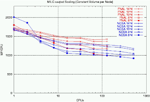
Figure 5: Performance of the MILC asqtad inverter on the T2 cluster (MILC code v6) and on the Pion cluster (MILC code using QDP, optimized by James Osborn). From Ref. [18].

Two more lessons can be drawn from asqtad inverter benchmarks on the T2 cluster displayed in Fig. 6 [24].

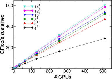
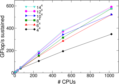
Figure 6: Performance of the MILC asqtad inverter on the T2 cluster using only a single CPU per motherboard (left) and using both CPUs (right) [24].

First, once the local volume is as small as $4^{4}$, the sustained performance drops significantly. Thus, even with an expensive, low-latency network such as Infiniband, strong scaling is limited. (To be fair, a local volume of $6^{4}$ is quite reasonable for most problems.) Second, the performance is roughly the same whether a single or both CPUs are used, i.e., the second Xeon is essentially useless in this case. This is due to the fact that with the chipset used on that cluster, the memory bandwidth is already saturated by a single CPU. (The Opteron with its memory controller on the chip would not have this problem.) Finally, weak-scaling curves for the domain-wall fermion (DWF) inverter (written in assembler by Andrew Pochinsky) are presented in Fig. 7 [25].

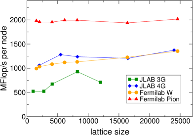
Figure 7: Weak scaling of the DWF inverter on four different PC clusters [25]. The peak performances per node in MFlop/s are 5300 (3G), 5600 (4G), 4800 (W), and 6400 (Pion). The labels on the horizontal axis correspond to the global 4-dimensional lattice size $V_{4}$, and the 5-dimensional lattice size is $V_{4}\times 16$.

The observation here is that with roughly comparable single-node performance, the Infiniband cluster obtains much higher sustained performance.

What processor/network combination provides the best price-performance ratio is a function of time. The US cluster community currently considers P4/Infiniband to be optimal. Other groups might (justifiably) have different preferences, see, e.g., the Opteron/Gig-E solution in Wuppertal. The 4G cluster at JLAB currently sustains 650 GFlop/s on the DWF inverter with a local lattice size of $8^{4}\times 16$, which translates into a cost-effectiveness of $1.1 per sustained MFlop/s in single precision (twice that for double precision). In the future, one hopes to sustain 1-2 TFlop/s on $\sim$1,000 nodes at a cost-effectiveness of $1 per sustained MFlop/s (single precision). The additional cost for power and cooling is estimated to be about 5% of the purchase price per year.

4.3 Custom-designed machines

As mentioned in Sec. 2, lattice QCD is well suited for parallelization. It is possible to design special-purpose capability machines that make use of the simplifying features of lattice QCD to obtain superior scalability, i.e., high sustained performance on a very large number of nodes, at very low cost. (The Grape project [26] is an extreme example of this idea in another field, i.e., astrophysics.) This approach is sensible only if the overall hardware budget available to the lattice community is large enough so that the higher cost-effectiveness of such machines is not spoiled by the development costs. Fortunately, this is true, and therefore special-purpose machines have been and will continue to be developed. Most of the history of these machines is described in the Machines & Algorithm section of the yearly LATTICE proceedings. Here, we will concentrate on the two latest machines, apeNEXT and QCDOC.

4.3.1 apeNEXT

The apeNEXT computer was designed and developed by a collaboration of INFN Ferrara and Rome, DESY Zeuthen and the Université de Paris-Sud, Orsay. It is the successor of earlier APE machines (APE, APE100, APEmille) and was presented at last year’s conference [27]. Further details can be found in Ref. [28]. The heart of the machine is a custom ASIC, the J&T processor, whose FPU can execute 8 Flops (a complex $a\times b+c$ operation) per clock cycle. Running at 160 MHz, this corresponds to a peak performance of 1.3 GFlop/s. The apeNEXT chip is shown in Fig. 8.

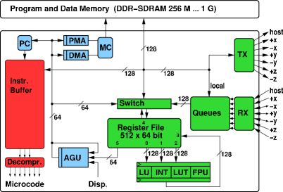
Figure 8: Block diagram of the J&T processor, the basic building block of apeNEXT. Taken from Ref. [28].

In addition to the FPU, it contains a 64 kB instruction buffer (as in the case of the Itanium, see Sec. 4.1.1, the VLIW idea is used), 10 kB of prefetch queues, a 4 kB register file, a controller for external memory with a bandwidth of 2.6 GB/s, and the communications hardware with DMA capability. The topology of the network is a three-dimensional torus with nearest-neighbor connections, allowing concurrent send and receive along any of the directions with a bandwidth of about 125 MB/s per link and direction.

As for the physical design of the machine, 16 daughterboards containing one ASIC each are mounted on a so-called processing board, which in addition contains an FPGA (field-programmable gate array) for the handling of global signals and an I2C interface. A backplane holds 16 processing boards, and a rack consists of two stacked backplanes, i.e., of 512 nodes. The footprint of a rack is less than 1 m², and the power consumption has been measured to be about 8.5 kW per rack.

apeNEXT can be programmed in TAO (a Fortran-like language specific to APE machines), in C (with an lcc-based compiler written by the apeNEXT team), or in SASM (high-level assembler). The TAO and C compilers are stable, but work is ongoing to improve code efficiency.

Unfortunately, due to an error made by the chip manufacturer, the apeNEXT project was somewhat delayed so that application code benchmarks could not be obtained yet on large machines. Currently, single-node performance is 54% of peak for the Wilson Dslash (hand-coded in assembler) and 37% for the TAO-based clover CG (the latter number is expected to go up with further optimization). A benchmark of the apeNEXT network performance is displayed in Fig. 9, where the total ping-ping and ping-pong latencies for a single bidirectional link are plotted as a function of the packet size.

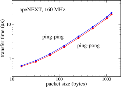
Figure 9: Measurements of the total ping-ping and ping-pong latencies as a function of the packet size for a single bidirectional link of apeNEXT at 160 MHz [29]. The benchmarks were written in SASM, use only registers and run in cache.

As can be seen from the figure, the ping-pong latency of the network is at least 500 ns, but most of this can be hidden, except in the case of global sums. A global sum takes $2(N_{x}+N_{y}+N_{z}-3)$ steps of $\sim$ 30 cycles each on an $N_{x}\times N_{y}\times N_{z}$ processor mesh, so on 1,024 nodes a global sum takes about 11 $\upmu$s. Strong-scaling numbers do not exist yet for the reasons mentioned above, but the machine should perform close to linear scaling since (a) the communications overhead for the Wilson Dslash is only 4% on a local volume of $2^{3}\times 16$ and (b) the global sums have no significant impact on the performance on machines with up to 4,096 nodes.

A short update on the progress of apeNEXT: a 512-node and a 256-node prototype rack using version A of the ASIC are running stably, and two 512-node racks using version B of the ASIC have been assembled and tested, with a target frequency of 160 MHz. The physics production codes are running with almost no modifications with respect to APEmille, but further optimization is needed to reach the efficiency of the benchmark kernels.

The following installations of apeNEXT are planned: 12 racks INFN, 6 racks Bielefeld, 3 racks DESY, and 1 rack Orsay. Based on a 160 MHz clock rate, the peak performance of a rack is 0.66 TFlop/s. The price is 0.60 Euro per peak MFlop/s [30], so the cost-effectiveness is about 1.2 Euro per sustained MFlop/s.

4.3.2 QCDOC

The QCDOC (QCD On a Chip) computer is a successor of the QCDSP machine [31] and was developed by a collaboration of Columbia University, the UKQCD collaboration, the RIKEN-BNL Research Center, and IBM Research. It has been discussed in detail at last year’s conference [32], and further material can be found in Ref. [33]. The architecture of the machine is based on the QCDOC ASIC, shown schematically in Fig. 10.

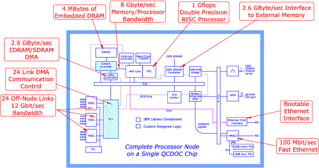
Figure 10: Block diagram of the QCDOC ASIC. Note that the peak performance and the memory and network bandwidths are based on a 500 MHz clock.

It contains a number of elements from IBM’s technology library (e.g., PowerPC 440 embedded CPU core, 64-bit FPU with one FMA per cycle, 4 MB embedded DRAM, memory controller, Ethernet controller, and high-speed serial links for the communications network) as well as custom-designed logic optimized for lattice QCD (e.g., serial communications unit with DMA capability, prefetching EDRAM controller, and bootable Ethernet-JTAG interface). Running at a conservative clock frequency of 400 MHz, its peak performance is 0.8 GFlop/s. The network has the topology of a six-dimensional torus with nearest-neighbor connections. As in the case of apeNEXT, concurrent send and receive is possible along any of the directions. The extra dimensions can be used to divide the machine into smaller partitions in software.

Two ASICs are mounted on a daughterboard, and 32 daughterboards are mounted on a motherboard. The motherboards can either be put in an air-cooled crate (8 each) or in a water-cooled cabinet (16 each). The footprint of a crate or a cabinet is about 1 m², and the power consumption is about 8 kW per cabinet.

There are currently five QCDOC installations: 14,720 nodes at Edinburgh (UKQCD), 14,140 nodes at BNL (USQCD), 13,308 nodes at the RIKEN-BNL Research Center, 2,432 nodes at Columbia University, and 448 nodes at the University of Regensburg.

QCDOC can be programmed in C, C++, or PowerPC assembler. There are two sets of compilers available, the free gcc/g++ and IBM’s commercial xlc/xlC. The latter produce faster code, but since critical kernels are available in assembler the GNU tools are generally sufficient.

We first present two benchmarks measuring the network performance of QCDOC. (Most of the benchmarks presented in this section were obtained by P.A. Boyle, with the exception of the asqtad performance in Table 3, which was obtained by C. Jung.) Figure 11 shows the aggregate actual bidirectional bandwidth obtained as a function of the message size and the number of active links.

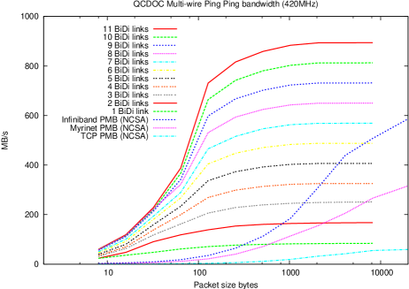
Figure 11: Measurements of the actual bidirectional bandwidth obtained on the QCDOC network at 420 MHz as a function of the message size and the number of active links. Also shown are the bandwidths obtained with three commercial networks (Infiniband, Myrinet, and Gbit Ethernet).

The maximum bidirectional bandwidth (including protocol overhead) at 420 MHz is 84 MB/s per link. Two points to note are that the multi-link bandwidth is comparable to the memory bandwidth and that a single link obtains 50% of the maximum bandwidth already on very small packets (32 bytes).

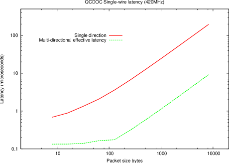
Figure 12: Total ping-ping latency for a single direction and multi-directional effective latency obtained on the QCDOC network at 420 MHz as a function of the message size.

Figure 12 shows the total ping-ping latency at 420 MHz for a single link as a function of the message size. Also shown is the multi-directional effective latency, which is obtained by transmitting in 12 directions simultaneously and dividing the transfer time by 12.

The network performance of QCDOC is reflected in the strong-scaling benchmark shown in Fig. 13.

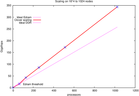
Figure 13: Strong-scaling benchmark for the sustained performance of the clover conjugate gradient on QCDOC at 420 MHz. The global volume is $16^{4}$.

Also shown are the ideal (i.e., linear) scaling curves when the data are located in on-chip (EDRAM) or off-chip (DDR) memory. We observe superlinear scaling when the problem moves from DDR to EDRAM, and linear scaling afterwards. On 1,024 nodes, the global volume of $16^{4}$ used in this benchmark corresponds to a local volume of $2^{2}\times 4^{2}$. The same sustained performance can be expected on 16,384 nodes using a $32^{4}$ global volume.

The sustained performance of various lattice QCD applications at 420 MHz for a local volume of $4^{4}$ is displayed in Table 3.

Action	# Nodes	matrix$\times$vector	CG performance
Wilson	512	44%	39%
Asqtad	128	42%	40%
DWF	512	46%	42%
Clover	512	54%	47%

Table 3: Lattice QCD application code performance on QCDOC in percentage of peak for a local volume of $4^{4}$.

Additional results can be found in the second paper of Ref. [32]. The author was unable to obtain updated benchmarks on larger machines since those machines are busy producing physics results. There are currently three RHMC jobs (with different quark masses) running on 4,096 nodes each in the US and the UK. The sustained performance of these jobs is only about 35% of peak since (a) the local volume of $6^{3}\times 2\times 8$ does not fit in EDRAM and (b) the linear algebra required for the multi-shift solver is running from external memory. Nevertheless, the total sustained performance of each of these jobs is over 1.1 TFlop/s. The two-flavor DWF inverter, which is part of the RHMC algorithm, sustains 40% of peak. When going from 1,024 to 4,096 nodes, superlinear scaling was observed since part of the problem moved into EDRAM and since there was no noticeable degradation from the communications overhead.

A 12-rack machine consisting of 12,888 nodes has a peak performance of 10 TFlop/s at 400 MHz. The price is $0.45 per peak MFlop/s [34], resulting in a cost-effectiveness of about $1.1 per sustained MFlop/s. The additional cost for power and cooling is less than 2% of the purchase price per year.

5 Speculations on future machines

Parallelization is the wave of the future, and not just in the field of high-performance computing. The increased power density and the associated heat dissipation problem is a major issue in the chip manufacturing industry, which sets a limit on the clock frequencies that can reasonably be achieved under normal operating conditions. The way out of this problem, which is already being taken by most of the major players, is to put multiple CPU cores on a single chip. While one could in principle run independent jobs on these cores, this will become increasingly difficult as the number of cores per chip increases since (a) the memory (and network) bandwidth will not be sufficient for many independent jobs and (b) the total amount of memory per chip would have to be very large (e.g., if we assume that a typical application requires 1 GB of memory, a chip with 32 cores would require 32 GB of memory, which is not just a technological challenge but also prohibitively expensive). On-chip parallelization would overcome these problems since the memory requirements per core, in terms of both bandwidth and amount, would be correspondingly smaller. Hardware designers dream of automatic parallelization (i.e., the detection of dependencies) in hardware, similar to the idea of dynamic instruction scheduling in superscalar RISC CPUs, see Sec. 4.1.1. However, it is not clear how practicable this approach is, and therefore a more conservative approach is to adjust the programming models to make efficient use of multi-core chips. What is necessary is more fine-grained parallelism on the chip. To get an idea of what is meant by this phrase, imagine a situation where the local volume per core is less than one site, i.e., the loops associated with a single site are distributed among several cores. Application code dealing with such a situation would probably contain a mixture of pthreads, OpenMP, and MPI (or similar implementations of the corresponding concepts), and data dependencies would have to specified by hand (e.g., in the form of compiler directives as in the case of OpenMP). The challenge to the system programmer is to write libraries that hide these details from the general user, and it will be interesting to see how this challenge is met in the future. Of course, lean software is essential to obtain as much performance as possible from such multi-core chips.

Will custom-designed chips continue to play a role lattice QCD? One of the problems facing chip designers are the very high NRE (non-recurring engineering) costs of large ASICs, which can be on the order of a few $$10^{6}$ or so. This is not a life-or-death issue for chips that will be manufactured in large volumes. However, for a dedicated lattice QCD chip of which only a few 10,000 units will be made, the NRE costs would represent a non-negligible fraction of the total cost. In addition, the financial risk associated with a possible re-spin of the chip would be very high. Some of the possibilities to deal with this issue are (a) to collaborate with a big company (such as IBM in the case of QCDOC), (b) to use FPGAs in the development phase, or (c) to combine a commercial processor with a custom-designed network ASIC (as in the case of QCDSP). (For an implementation of the Wilson-Dirac operator on an FPGA, see Ref. [35].)

There is no doubt that PC clusters will contribute a major percentage of the computing power available for lattice QCD. Since PC clusters are used by many communities, the market is sufficiently large to drive improvements in cluster hardware at all fronts (processors, memory bus, chipsets, network interfaces, etc.). For example, a custom-designed three-dimensional interconnect architecture for PC clusters called APENet was presented at this conference [36]. A continuous software effort is necessary to get maximum performance out of the new architectures. It will be interesting to see how multi-core chips perform in a cluster environment.

Let us mention concrete proposals for new machines and speculate on some possible future projects.

• PC cluster upgrades are planned at JLAB (a clone of the 260-node Fermilab Pion cluster will go online in the spring of 2006) and at Fermilab (an Infiniband cluster with $\sim$1,000 processors, either $\sim$500 dual Xeons or $\sim$1,000 single Pentiums depending on price/performance at the time, will be installed in the fall of 2006) [25].

• Ukawa presented the plans of the Center for Computational Sciences at Tsukuba for their new PACS-CS machine, which will consist of 2,560 2.8 GHz Intel Xeon processors connected by a three-dimensional Gbit-Ethernet-based hyper-crossbar network. The peak performance of the machine is 14.3 TFlop/s, and it should be operational by July 2006. For details, see Ref. [37].

• KEK is currently collecting bids for a machine with at least 24 TFlop/s peak performance, to be operational by March 2006.

• A successor to QCDOC is under consideration, but concrete decisions have not yet been made.
  

• IBM is working on a successor to BG/L called BlueGene/P. This machine is supposed to break the PFlop/s barrier, but details on the architecture and the schedule have not yet been released.

• Fujitsu has announced plans to build a machine with a peak performance of 3 PFlop/s by 2010/11. This machine is supposed to use optical switching technology that has yet to be developed.

• The Japanese technology ministry is discussing plans to develop a 10 PFlop/s machine by 2010/11, with a projected budget on the order of $10^{11}$ yen (roughly $$10^{9}$ depending on the exchange rate). A budgetary decision was supposed to be taken by the end of August but has been delayed because of the early elections in Japan.

Another interesting question is whether the Cell chip [38] can be used for lattice QCD simulations. This is a gaming chip made by IBM for Sony and will power the Playstation 3. It contains a new PowerPC CPU and 8 FPUs, each of which has 256 kB of private memory. There is also 512 kB of L2-cache on chip. Each FPU can perform 4 single-precision FMAs per clock cycle. At the nominal clock frequency of 4 GHz, this translates into a peak performance of 256 GFlop/s (single-precision) per chip. Double-precision performance is estimated to be about 10 times slower. The memory interface (Rambus XDR) has a bandwidth of 25.2 GB/s, and the I/O interface (Rambus FlexIO) provides a total bandwidth of 76.8 GB/s (44.8 in, 32 out). The big question for lattice QCD applications is whether the memory system can keep the FPUs fed. Since the chip has not yet been released and details are hard to come by, only rough guesstimates are possible. Based on bandwidth estimates, a sustained single-node performance on the order of 15-20% might be achievable [39]. Note, however, that the arithmetic is not IEEE-compliant (the FPUs always round down). This introduces a bias in the numerical Monte Carlo simulations, which has to be eliminated by careful fix-up code. In practice, this issue will set a limit on the amount of application code that can take advantage of the high performance of the FPUs.

6 Conclusions

The machines that have been custom-designed for lattice QCD (apeNEXT and QCDOC) are still the leading capability machines in our field. They currently provide the best price-performance ratio (about $1 per sustained MFlop/s in the case of QCDOC) for large-scale lattice QCD applications. PC clusters are competitive as capacity machines and might also be used as capability machines in the future as cluster scalability improves. If single precision is sufficient, their cost-effectiveness is already comparable to that of the custom-designed machines. Commercial supercomputers are typically much less cost effective. It would not be a good idea for a lattice group to purchase such a machine, but if computing time can be obtained in a computing center it should of course be used. BlueGene/L is an interesting alternative, as it is both a commercial product and rather close to the QCDOC architecture. To break even with QCDOC, the purchase price for a rack of BG/L should not be more than about $1 million. (Apparently, IBM has also been offering computing time on BG/L at a price of $6.7 million per rack and year [25].) Looking into the future, multi-core chips will become prevalent very soon. All three avenues (custom-designed machines, PC clusters, and commercial supercomputers) should continue to be explored, and all three of them are likely to remain important.

Designing or purchasing the best possible hardware is not sufficient. Lean and efficient software is absolutely necessary to obtain high performance. The trend towards on-chip parallelization will pose new challenges to the programmer, and the programming models will have to change to make maximum use of multiple cores per chip. High-performance code will most likely contain a combination of pthreads, OpenMP, and MPI. It will be very interesting to follow the future developments in this area.

References

- [1] see, e.g., T.A. Kennedy, Nucl. Phys. B (Proc. Suppl.) 140 (2005) 190 [hep-lat/0409167] and references therein
- [2] M. Hasenbusch et al., Nucl. Phys. B (Proc. Suppl.) 129 (2004) 847 [hep-lat/0309149]
- [3] P.A. Boyle, in preparation
- [4] http://www.physics.utah.edu/~detar/milc
- [5] http://www.jlab.org/~edwards/chroma
- [6] http://qcdoc.phys.columbia.edu/chulwoo_index.html
- [7] http://www.fermiqcd.net
- [8] http://www.usqcd.org
- [9] S. Aoki et al., Annual Report of the Earth Simulator Center (2004), http://www.es.jamstec.go.jp/esc/images/annualreport2003/pdf/project/chapter4/4-04ukawa.pdf
- [10] http://www.uni-koeln.de/rrzk/kompass/104/k1045.html
- [11] G. Bhanot, D. Chen, A. Gara, and P. Vranas, Nucl. Phys. B (Proc. Suppl.) 119 (2003) 114 [hep-lat/0212030]
- [12] G. Bhanot, D. Chen, A. Gara, J. Sexton, and P. Vranas, Nucl. Phys. B (Proc. Suppl.) 140 (2005) 823 [hep-lat/0409042]
- [13] IBM Journal of Research and Development 49 (2005)
- [14] T. Lippert, Nucl. Phys. B (Proc. Suppl.) 129 (2004) 88 [hep-lat/0311011]
- [15] D.J. Holmgren, Nucl. Phys. B (Proc. Suppl.) 140 (2005) 183 [hep-lat/0410049]
- [16] D.J. Holmgren, PoS (LAT2005) 105
- [17] R.G. Edwards, http://online.kitp.ucsb.edu/online/lattice_c05/edwards
- [18] D.J. Holmgren, http://lqcd.fnal.gov/allhands_holmgren.pdf
- [19] F. Csikor et al., Comput. Phys. Commun. 134 (2001) 139 [hep-lat/9912059]
- [20] M. Lüscher, Nucl. Phys. B (Proc. Suppl.) 106 (2002) 21 [hep-lat/0110007]
- [21] A. Pochinsky, Nucl. Phys. B (Proc. Suppl.) 140 (2005) 859
- [22] http://crd.lbl.gov/FTG/MVIA/mvia.shtml
- [23] http://www.lqcd.org/qmp
- [24] S. Gottlieb, private communication
- [25] D.J. Holmgren, private communication
- [26] http://www.astrogrape.org
- [27] F. Bodin et al., Nucl. Phys. B (Proc. Suppl.) 140 (2005) 176
- [28] F. Bodin et al., hep-lat/0306018, hep-lat/0309007
- [29] H. Simma, private communication
- [30] L. Tripiccione, private communication
- [31] R.D. Mawhinney, Parallel Comput. 25 (1999) 1281 [hep-lat/0001033]
- [32] P.A. Boyle et al., Nucl. Phys. B (Proc. Suppl.) 140 (2005) 169, 829
- [33] P.A. Boyle, C. Jung, and T. Wettig, hep-lat/0306023; P.A. Boyle et al., IBM Journal of Research and Development 49 (2005) 351
- [34] N.H. Christ, private communication
- [35] O. Callanan, A. Nisbet, M. Peardon, and D. Gregg, PoS (LAT2005) 102
- [36] R. Ammendola et al., PoS (LAT2005) 100
- [37] A. Ukawa, PoS (LAT2005) 111
- [38] There is very little official information available on the Cell chip. The numbers quoted in the text were taken from http://www.realworldtech.com/page.cfm?ArticleID=RWT021005084318
- [39] P.A. Boyle, private communication